Received 4 May 2016; accepted 12 July 2016; published 15 July 2016

ABSTRACT

A five-mode truncation of the Navier-Stokes equations for a two-dimensional incompressible fluid on a torus is studied. Its stationary solutions and stability are presented; the existence of attractor and the global stability of the system are discussed. The whole process, which shows a chaos behavior approached through an involved sequence of bifurcations with the changing of Reynolds number, is simulated numerically. Based on numerical simulation results of bifurcation diagram, Lyapunov exponent spectrum, Poincare section, power spectrum and return map of the system, some basic dynamical behavior of the new chaos system are revealed.

Keywords:

The Navier-Stokes Equations, Strange Attractor, Lyapunov Function, Bifurcation, Chaos

1. Introduction

In recent years, many scholars were enthusiastic for the stability and the bifurcation of truncated model of the Navier-Stokes equations [1]-[5]. A pioneering work by Lorenz [6] of 1963, concerning the Saltzman equations for convection between plates, represents the first attempt to study the partial differential equations that govern a fluid flow through truncation of a suitable Fourier expansion to a finite number of components (“modes”). Later in the twentieth century, Valter Franceschini made a further expansion in this research field and worked with other scholars to study the Navier-Stokes equations. They consider the following plane incompressible Navier-Stokes equations on the torus, the velocity field, the pressure and (periodic) volume force. is expanded in Fourier series on a torus. Some model Lorenz-like equations have been proposed, then they have studied three-dimensional Navier-Stokes, the equation in and obtained somenonlinear system, and discussed these complex system in detail in [3]-[5].

In this paper, we expand the plane incompressible Navier-Stokes equations in Fourier series on a torus and obtain a new five-mode equation. Dynamical behaviors of this new chaotic system, including some basic dynamical properties, bifurcations, and routes to chaos, etc., have been investigated both theoretically and numerically by changing Reynolds number. Our purpose is to study how the phenomena of the model changes when the modes in the truncation are changed. The existence of attractor and the global stability of the equations have been firmly verified and these theories can be used in other similar model. Furthermore, some dynamical behavior features of the new chaos system in a certain range of the Reynolds number, such as bifurcation diagram, Lyapunov exponent spectrum, Poincare section, power spectrum and return map, are presented.

We expanded, , in Frourier series, and take as the set of vectors and their opposites. With a lot of calculation, we obtain the following five-mode Lorenz-like system

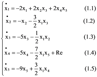(1)

Accordingly, we get the new five-mode nonlinear equation, which is similar to the Lorenz equation. We call it a Lorenz-like equation. By changing both the signs of and, the property of the equations is unchanged. This indicates that system (1) has following symmetry property

.

2. The Stationary Solution and Their Stability Properties

In the following we linearize the nonlinear Equation (1) and discuss the stability of its stationary solutions.

a) For, there is only one stationary solution. Substituting

the stationary solution into the Jacobian matrix we obtain the characteristic equation of Jacobian matrix

For, since all eigenvalues of the Jacobian matrix are negative, the stationary solution is stable (this is a particular case of general results on the theory of the Navier-Stokes equations [7]), and numerical evidence suggests that the is a global attract or for all.

b) For, there are 3 stationary solutions: the old one, which has become unstable

as a consequence of the crossing of the imaginary axis by one of the eigenvalues of the Jacobian matrix) and two additional as follow

.

By a similar discussion we get the characteristic equation of Jacobian matrix at is:

(2)

owing to roots of the characteristic Equation (2) have a negative real part, stationary solution are stable. Numerical evidences indicate that any randomly chosen initial data is attracted by them, so they are global attractors. When

c) For, there are 7 stationary solutions: the old ones, , and, with components

.

The first three are now always unstable, while the new four are stable for and numerically they attract any randomly chosen initial data. At the fours table stationary solutions become unstable because a pair of complex conjugate eigenvalues crosses the imaginary axis, and four stable periodic orbits around the fixed points arise via a Hopf bifurcation, we will give a detailed discussion in the Section 4.

3. The Existence of Attractor and Analysis of Global Stability

In the following, we discuss the existence of attractor of the system (1), assume that

, by calculating we get. Using the Gronwall inequality [8], we get. Therefore, we have. If big enough,

sphere is an not only functional invariant set but also absorbing set. As a result the system (1) has the global attractor [8] [9].

We construct a following Liapunov function of the system (1):

(3)

Setting, obviously, when k is a positive constant, it represents a sphere, which is labeled as E. By calculating we obtain the following derivative

(4)

Obviously, represents an ellipsoid in H, which is labeled as C. From (4) we know that on outside of C, on C, and inside of C. If k is big enough, E will include C. Therefore, from (4) we know that, on outside of C. From the Liapunov

theory we know that the orbits of system (1) will enter E. Namely E is the trapping region of the equations (1). Though the stationary solutions, , and are all unstable, the system (1) still has the global stability, orbits of system (1) contract into the trapping region and oscillates in the trapping region. Finally the orbits form an invariant set in the trapping region, which is called the strange attractor.

4. Numerical Simulation

In this section we present the numerical experiment results.

1) For Re < R3 = 52.785…, the stationary solutions of system (1) is stable, Numerical evidences indicate that any randomly chosen initial data is attracted by one of them, so they are global attractors.

2) At Re = R3 = 52.785… the four stable stationary solutions become unstable because a pair of complex conjugate eigenvalues of Jacobian matrix at stationary point crosses the imaginary axis, each of the four stable fixed points generated by the preceding bifurcations loses stability undergoing a Hopf bifurcation, and each generates a stable periodic orbit (hence foursymmetric orbits are generated), and four stable periodic orbits around the fixed points arise via a Hopf bifurcation (Figure 1) are stable up to Re = R4 = 55.36 ∙∙∙ and numerical results shows that they attract any point chosen at random.

3) At Re = R4 = 55.36 ∙∙∙, the periodic orbits lose stability. As predicted by the general theory of bifurcation [7], Numerical evidences indicate that each one of the periodic orbit gives rise to a new periodic orbit, the new orbits are very similar in shape to the previous ones, only they wind up twice (Figure 2). With the increasing of

the Reynolds number Re, the number of periodic orbits also increases, the computer simulation shows that other similar bifurcations take place at Re = R5 = 55.365 ∙∙∙, Re = R6 = 55.40 ∙∙∙ and Re = R7 = 55.60 ∙∙∙, each time the new orbits wind up around the fixed points twice, at this point, the system is in a state of quasi-periodic. the sequence of period doubling bifurcations should accumulate (according to Feigenbaum’s theory); in another region of phase space a pair of periodic orbits (one stable and one unstable) are created, therefore, a hysteresis (i.e., coexistence of attractors) phenomenon appears.

4) As discussed above, at Re = R7 = 55.64 ∙∙∙, a new kind of periodic orbit appears. Each of the previous four orbits bifurcates into anew orbit, the new orbits wind up around two of the fixed points, instead of only one like the previous ones. More precisely there are two orbits winding around and and the other two around and (one stable and one unstable) (Figure 3).

The attraction basin of the stable periodic orbit rapidly extends, as Re grows within a very small interval. While Re in this interval a hysteresis phenomenon occurs and some initial data are attracted by the new stable orbit and others are attracted by the doubling periodic orbits (see Figure 3). Soon the attraction basin of the new orbit appears to swallow the region where the doubling periodic should be located. A “collision chaos” seems to take place.

5) The stable periodic orbit become unstable at Re = R8 = 55.76 ∙∙∙, increasing Re we have a sequence of bifurcations in which each time the period doubles and the number of loops around each fixed point doubles. We found four further bifurcation points of such nature, for the following values of Re:Re ; 55.80..., Re ; 55.84, Re ; 55.92. Since the period doubles each time and the orbits become increasingly intricate requiring higher precision, we did not look for further bifurcations. So we cannot definitely state whether we have just a finite number of bifurcations and the only obstacle to observe more seems to be the numerical precision needed, then the strange attractor appears, namely, the period doubling bifurcations transition into chaos (Figure 4 & Figure 5).

6) Figure 6 shows bifurcation diagrams of the system (1). Figure 7 shows the corresponding largest Lyapunov exponents. The periodic motions generated by the period doubling bifurcation continue to double in ever faster succession (as Re grows) eventually generating a chaotic attracting set. Moreover, these bifurcation diagrams show self similarity.

7) Figures 8-10 show Poincare section, return map and power spectrum of the system (1) at Re = 57.95. They indicate chaos feature of the new system (1).

8) From bifurcation diagrams Figure 7, we find that the chaotic region contains periodic-orbit windows of

varying width, the strange attractors and limit cycles appear alternately at some Reynolds number. Through more delicate and difficult calculation we obtain the following details: at Re = 58.88... the strange attractor shrinks into a symmetrical limit cycles (Figure 11), at Re = 59.90..., the limit cycles become unstable and the periodic orbits generated by the period doubling bifurcation continue to double in ever faster succession eventually generating a chaotic attracting set (Figure 11). At Re = 68.48..., the strange attractor shrinks into a symmetrical limit cycles again, if followed backwards with decreasing Re, this bifurcation is an “inverse” bifurcation.

5. Conclusion

This paper has presented and studied a five-mode Lorenz-like system of the Navier-stokes equations for a two- dimensional incompressible fluid on a torus. Dynamical behaviors of this new chaotic system, including some basic dynamical properties, bifurcations, and routes to chaos, etc., have been investigated both theoretically and numerically by changing Reynolds number. We have found period-doubling bifurcations to chaos, intermittent scenario, periodic windows, hysteresis and coexistence of periodic attractors. The chaotic behavior was discussed with the aid of bifurcation diagram, Lyapunov exponent spectrum, Poincare section, power spectrum and return map. Furthermore, the existence of attractor and the global stability of the equations have been firmly verified and our theories and methods can be used in other similar systems.

Acknowledgements

We thank the editor and the referee for their comments. Research works are subsidized by the National Nature Science Foundation of China (11572146), the funds for education department of Liaoning Province (L2013248) and science and technology funds of Jinzhou city (13A1D32).

Cite this paper

Heyuan Wang, (2016) A Five-Mode System of the Navier-Stokes Equations on a Torus. Journal of Applied Mathematics and Physics,04,1245-1253. doi: 10.4236/jamp.2016.47130

References

- 1. Wang, H.Y. (2012) Dynamical Behaviors and Numerical Simulation of Lorenz Systems for the Incompressible Flow between Two Concentric Rotating Cylinders. International Journal of Bifurcation and Chaos, 22, 1-11. http://dx.doi.org/10.1142/S0218127412501246
- 2. Wang, H.Y. (2015) The Chaos Behavior and Simulation of Three Model Systems of Couette-Taylor Flow. Acta Mathematica Scientia, 35, 769-779.
- 3. Franceschini, V., Inglese, G. and Tebaldi, C. (1988) A Five-Mode Truncation of the Navier-Stokes Equations on a Three-Dimensional Torus. Computational Mechanics, 3, 19-37. http://dx.doi.org/10.1007/bf00280749
- 4. Franceschini, V. and Zanasi, R. (1992) Three-Dimensional Navier-Stokes Equations Trancated on a Torus. Nonlinearity, 4, 189-209. http://dx.doi.org/10.1088/0951-7715/5/1/008
- 5. Franceschini, V. and Tebaldi, C. (1984) Breaking and Disappearance of Tori. Communications in Mathematical Physics, 94, 317-329. http://dx.doi.org/10.1007/BF01224828
- 6. Lorenz, E.N. (1963) Deterministic Nonperiodic Flow. Journal of the Atmospheric Sci-ences, 20, 130-141. http://dx.doi.org/10.1175/1520-0469(1963)020<0130:DNF>2.0.CO;2
- 7. Ladyzhenskaya, O.A. (1969) The Mathematical Theory of viscous Incompressible Flows. Gordon and Breach, New York.
- 8. Li, K.T. and Ma, Y.C. (1992) The Hilbert Space Method of Math and Physics Equations. Xi’an Jiaotong University Press, Xi’an.
- 9. Hilborn, R.C. (1994) Chaos and Nonlinear Dynamics. Oxford University Press, London.