Open Access Library Journal
Vol.03 No.01(2016), Article ID:68177,8 pages
10.4236/oalib.1102313
Study on Numerical Simulation of Oil-Water Phase Non-Darcy Flow in Low-Permeability Reservoirs
Rongqiang Li*, Jianzhong Wang
China University of Petroleum, Qingdao, China

Copyright © 2016 by authors and OALib.
This work is licensed under the Creative Commons Attribution International License (CC BY).
http://creativecommons.org/licenses/by/4.0/


Received 30 December 2015; accepted 14 January 2016; published 18 January 2016

ABSTRACT
Based on the basic laws of non-Darcy seepage in low permeability media as well as dynamic permeability, a dynamic function of permeability is derived. On this basis, factoring in the effect of the non-linearity and the starting pressure gradient, a piecewise numerical simulation model was established for low permeability reservoirs and through discretization, a numerical model was obtained. According to the results of the simulation test, this model and method reflect well the seepage in low permeability reservoirs, expressing more objectively the influence of the starting pressure gradient and the non-linearity.
Keywords:
Low Permeability Reservoir, Non-Darcy Flow, The Threshold Pressure Gradient, Numerical Simulation
Subject Areas: Chemical Engineering & Technology

1. Introduction
Compared to intermediate and high permeability reservoirs, low permeability reservoirs have larger specific surface, smaller pores, and extremely narrow pore throat. The abnormal pore structure highlights the existence of the solid-liquid boundary layer, the fluid’s non-Newtonian effect, and the capillary force, which makes the fluid’s seepage deviate from the Darcy’s law [1] - [3] . The main features of this deviation include the existence of the starting pressure gradient and the non-linearity of the flow pattern with low pressure gradient. In recent years, low permeability reservoir has gradually become the main target of oil and gas field development, whereas the conventional software for numerical reservoir simulation lacks support for it.
The non-Darcy flow laws and mechanism of fluid in low permeable porous media once were the hot spot of research. However, these achievements are still in the development phase, far from perfect. Quasi-linear descriptions of the non-Darcy flow were used to approximately substitute for the non-linear pattern, and the influences of the starting pressure gradient were overestimated [4] - [8] . Bottoming on the analysis of non-Darcy seepage in low permeable media, this paper is built on the concept of dynamic permeability mentioned in Ref. [9] to establish the reservoir numerical simulation model to make an accurate description of the effect of non- linearity.
2. Non-Darcy Seepage in Low Permeability and Its Mathematical Description
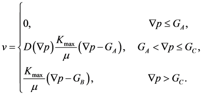
Changes in flow velocity in hypotonic medium as the driving pressure gradient increases is divided into three distinct phases, shown in Figure 1: (1) no-flow section (OA), the driving pressure gradient is very small, yet the fluid begins to flow; (2) nonlinear section (AD above), when the pressure gradient is greater than the value of the point A, the fluid begins to flow and the pressure gradient is often referred to as the starting pressure gradient (hereinafter, represented by GA). With the increase of the pressure gradient, the flow velocity changes non- linearly; (3) quasi-linear segment (DE section), when the pressure gradient increases to a certain extent, the flow curve gradually transits from a non-linear segment to a straight line segment. D is the point on the curve of transition from the non-linear segment to the straight line segment. Its pressure gradient is called the critical pressure gradient (hereinafter denoted by GC) corresponding to the critical permeability (hereinafter represented by Kmax). B is the intersection point of an extending DE and the pressure gradient axis, often referred to as threshold pressure gradient (hereinafter denoted by GB). The motion equation of the three different stages can be expressed:
 (1)
(1)
where in Ñp represents the pressure gradient (which herein refers to its mode), a, b, c are constants, and μ is the viscosity of the fluid. According to the concept of dynamic permeability, assuming the permeability of any point on the non-linear segment is K(Ñp), differentiate the nonlinear equation with respect to Ñp, and physically speaking, the derivative of this point is its mobility, namely:
 (2)
(2)
Therefore: ,
, .
.

Figure 1. Three stages of non-Darcy flow in low-permeability reservoir.
If define the dynamic function of permeability as:
 (3)
(3)
Then the dynamic permeability of the nonlinear segment is as follows:
 (4)
(4)
Then rewrite the motion equation of seepage in low permeability reservoirs as:
 (5)
(5)
As can be seen from the above equation, the introduction of dynamic function of penetration, enables the nonlinear seepage to be processed linearly.
3. The Mathematical Model for Numerical Simulation of Low Permeability Reservoir
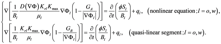
In reference to the black oil model, taking into account the water and oil phases have the same starting pressure gradient [10] , convert pressure into potential function ( ), and a three-dimensional, two-phase mathematical model of low permeability reservoir numerical simulation can be expressed as:
 (6)
(6)
In Equation (6), there are a total of four unknowns in the two equations involving the two phases of oil and water, two auxiliary equations are needed:
 (7)
(7)
For the above equation, the inner boundary condition can be fixed bottom hole pressure or fixed yield (injection volume); the closed outer boundary condition is ; initial conditions are
 ,
, .
.
For the above mathematical model, because the two-phase flow equation has two stages, namely the non- linear stage and the quasi-linear stage, when calculating phase identification must be carried out in order to select the appropriate equation. More specifically, first obtain the respective relationship between the minimum threshold pressure gradient, the critical pressure gradient and mobility, then compare the current pressure gradient value with the calculated starting pressure gradient and critical pressure gradient. The principle is similar to checking the identification plate (Figure 2).
4. The Numerical Model for Simulation of Low Permeability Reservoir
Due to the length limit, the non-linear equations are taken for example to present the discretization process. First derive a difference expression of item on the left side of the nonlinear equation. In order to simplify the equation, a linear differential operator is introduced:

Figure 2. Fluid flow stage discrimination diagram of low permeability reservoir.
 (8)
(8)
wherein:  is the coefficient of conductivity, where F is the geometrical factor, dependent on the mesh size and absolute permeability, independent of time. Since
  is only related to the pressure gradient of the grid, and not to pressure, before the calculation of each time step, the pressure gradient of each grid should be calculated to determine the flow phase of the fluid. If the flow is non-linear, then calculate
 . The implicit iterative scheme is used to derive the difference equation of the oil phase equation. For any time step from
  to
to , the parameter change between two iterations can be expressed as [11] - [13] :
 (9)
(9)
 in the above formula can be expressed as:
 (10)
(10)
Thus derive a difference expression of the oil phase equation and then expand it, while the right-hand side of the equation is differentiated:
 (11)
(11)
Similarly, considering the capillary pressure, the aqueous phase of the equation can be expressed as:
 (12)
(12)
where:  is the formation porosity under reference pressure, as a decimal;
  is rock compressibility, MPa−1.
In the calculations, mobility can be selected according to the usual “upstream rights” law; as for the selection of starting pressure gradient, because when the fluid flows from grid i + 1 to grid i, the first starting pressure gradient of grid i + 1 plays a dominant role, it can also be determined using the “upstream right” method.
If:  then take
 ,
, 
If:  then take
 ,
, 
The discretization of the quasi-linear flow equation is basically the same as that of the nonlinear phase. For differential equations in potential gradient, there are component differential and mode differential methods. Similarly considering the influence of starting pressure gradient on the flow, herein consulted are the mode differential method of potential gradient and the corresponding algorithms in Ref. [7] .
5. The Method Testing and Results Analysis
5.1. Testing and Analysis with Theoretical Models
Realization of reservoir simulation software is a large and complex project. A set of Fortran source codes of conventional reservoir simulation software developed by earlier researchers were analyzed and adapted. Based on the original algorithm, when the non-Darcy flow is factored in, numerical simulation for hypotonic reservoir is realised. The software runs on 64-bit linux environment and for solving linear equations, needs PETSc (Portable Extensible Toolkit for Scientific Computation) support. For comparison, the altered software also has the function to simulate the quasi-linear non-Darcy flow.
In order to verify the correctness and rationality of numerical simulation method of low permeability reservoirs, the theoretical model of homogeneous reservoir with a five-point injection well network is established. In the model, both x and y directions are divided into 21 grids, z direction is divided into 5 grids. Assume the binomial coefficient in the nonlinear flow equation in low permeability reservoirs were a = 0.4, b = 0.4, c = −0.05; starting pressure gradient, pressure gradient and critical threshold pressure are respectively GA = 0.0003 MPa/m, GB = 0.00135 MPa/m, GC = 0.003 MPa/m. Set that the wells are operated with given injection rate, fixed- volume production, the calculated pressure field after five months (153 days) is shown in Figure 3.
As can be seen from Figure 3, there are remarkable differences among the simulated pressure fields (mesh layer 1) in accordance with different seepage laws. Results of the simulation based on classical Darcy’s laws show that, due to not considering the effects of starting pressure gradient and nonlinearity, compared to the other cases, the isobar is sparse and the pressure change is relatively mild (as shown in Figure 3(a)). Compare Figure 3(b) and Figure 3(c), the quasi-linear simulation results, compared to nonlinear simulation results, show more dense isobar, indicating greater pressure gradient between the injection and production wells. This is because the quasi-linear seepage law exaggerates the impact of starting pressure gradient while ignoring flow under low pressure gradient. The flatness of the simulated pressure distribution using nonlinear law is between Darcy and quasi-linear, consistent with the theory.
5.2. Testing and Analysis with Field Examples
In order to further test and verify the correctness of the proposed numerical simulation of low permeability reservoir, model of an actual reservoir is established, using data of a block of the Daqing Oilfield. The grid is divided into 38 × 26 × 6, the planar grid in the x direction is 48 m, in the y direction is 43 meters. There are six injection wells, 15 producing wells, their location shown in Figure 4. The flow pattern data is identical to the five-spot well pattern, and the wells are set to operate with fixed injection and fixed output.
Figure 5 shows respectively the reservoir pressure field of simulation based on Darcy’s law, the law of quasi- linear and non-linear after 153 days operation. It can be seen from the figure that, while maintaining the same oil production, the pressure changes according to Darcy’s law are small (Figure 5(a)); compare Figure 5(b) and Figure 5(c), it can be seen that, under the condition of the same oil yield, due to an overestimate of the impact of starting pressure gradient by the quasi-linear seepage law, compared to the non-linear law, the quasi-linear equations demonstrate greater pressure drop and more dramatic change in the pressure field.
The different flow laws to base the Numerical simulation on and whether or not to consider the starting pressure gradient, are bound to affect the injection and production of wells. Run the simulation based on respectively Darcy’s law, the quasi-linear law and non-linear law, the pressure distribution between the injection and production wells are derived. According to the results, the simulation based on Darcy’s law show a relatively flat
 (a)
(a)
 (b) (c)
Figure 3. Pressure distribution of simulated results based on different rule. (a) Darcy flow; (b) Quasilinear seepage; (c) Nonlinear flow.

Figure 4. Oil wells location map.
 (a)
(a)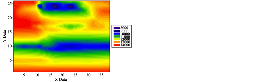
 (b) (c)
Figure 5. Pressure distribution of simulated results based on different rule. (a) Darcy flow; (b) Quasilinear seepage; (c) Nonlinear flow.
pressure distribution among injection and production wells, which is mainly due to an underestimate of the formation resistance; the simulation based on the law of quasi-linear flow show, due to an overestimate of the impact of the starting pressure gradient, more significant pressure variations between wells; simulation based on the nonlinear law show results that fall in between, which coincide with expectations.
6. Conclusions
The piecewise mathematical model described in this paper closely follows the basic rules of non-Darcy flow in low permeability, based on dynamic penetration thinking, uses the dynamic function of permeability to address the complex nonlinear issue with linear methods, and therefore, more objectively reflects the impact of non- linearity and starting pressure gradient. This model is more suitable for the numerical simulation of low permeability reservoirs than the existing Darcy and quasi-linear models. From the perspective of the simulation results, the model is consistent with theoretical expectations.
It should be noted that the scientificity of numerical reservoir simulation methods relies on the knowledge of the basic laws of oil and gas seepage. Non-Darcy flow theory in low permeability is still in the developing stage, so the models and methods adopted in this paper are also in a continuous exploration stage. Inevitably there will be some limitations or one-sidedness.
Cite this paper
Rongqiang Li,Jianzhong Wang, (2016) Study on Numerical Simulation of Oil-Water Phase Non-Darcy Flow in Low-Permeability Reservoirs. Open Access Library Journal,03,1-8. doi: 10.4236/oalib.1102313
References
- 1. Huang, Y.Z. (1997) Nonlinear Percolation Feature of Low Permeability Reservoir. Special Reservoir, 4, 9-14.
- 2. Iwere, F.O. and Moreno, J.E. (2006) Numerical Simulation of Thick, Tight Fluvial Sands. SPE Reservoir Evaluation & Engineering, 9, 374-381.
http://dx.doi.org/10.2118/90630-PA - 3. Xu, S.L., Yue, X.G., Hou, J.R., et al. (2007) Effect of Boundary Layer Fluid Flow in Low Permeability Reservoir Characteristics. Xi’an Petroleum University: Natural Science, 22, 26-28.
- 4. Guo, Y.C., Lu, D.T. and Ma, L.X. (2004) Low Permeability Reservoir Seepage Numerical Difference Method. Hydrodynamics Research and Development, 19, 288-293.
- 5. Su, H.J. (2004) A Three-Phase Non-Darcy Flow Formulation in Reservoir Simulation. SPE Asia Pacific Oil and Gas Conference and Exhibition, Perth, 18-20 October 2004, SPE: 88536.
http://dx.doi.org/10.2118/88536-ms - 6. Han, H.B., Cheng, L.S., Zhang, M.L., et al. (2004) Ultra-Low Permeability Reservoir in Consideration of Starting Pressure Gradient Physical Modeling and Numerical Simulation. Petroleum University: Natural Science, 28, 49-53.
- 7. Li, L., Dong, P.C., Zhang, M.L., et al. (2006) Ultra-Low Permeability Reservoir with Non-Darcy Flow Model and Its Application. Mechanics and Geotechnical Engineering, 25, 2272-2279.
- 8. Zhao, G.Z. (2006) Numerical Simulation of Three-Dimensional Three-Phase Flow Pressure Gradient Method Becomes Starts. Petroeum, 27, 119-128.
- 9. Yao, J. and Liu, S. (2009) Low Permeability Reservoir Well Test Interpretation Model Based on Dynamic Penetration Effect. Petroeum, 30, 430-433.
- 10. Li, A.F., Liu, M., et al. (2010) Pressure Gradient Variation in Low Permeability Reservoir Water Two-Phase Start. Xi’an Shiyou University, 25, 17-54.
- 11. Han, D.K., Chen, Q.L. and Yan, C.Z. (1993) Reservoir Simulation Basis. Petroleum Industry Press, Beijing.
- 12. Li, S.X. and Gu, J.W. (2009) Reservoir Simulation Basis. China University of Petroleum Press, Dongying.
- 13. Peaceman (1982) Reservoir Simulation Basis. Petroleum Industry Press, Beijing.
NOTES

*Corresponding author.