Received 25 December 2015; accepted 10 January 2016; published 13 January 2016

ABSTRACT

Based on an assumption of that the cosmological constant term in Einstein field equation can be modeled as a material medium, we propose the concept of cosmological acoustic wave (CAW). In the process, we will see: 1) By the dual framework of electromagnetic theory, it is possible to consider some implications of CAW, such as, the acoustic charge quantization, the unit spin of phonon, the mechanical meaning of acoustic current and the acoustic radiation. It shows that, besides the transverse and longitudinal waves, there should be a sort of adjoint waves without contribution to energy flows. 2) The electromagnetic-acoustic equations are applied in homogeneous and isotropic material media, which can help us to describe uniformly the electromagnetic-acoustic phenomena. 3) It will be verified that, the acoustic interaction is identical to the gravitational one in classical physics. This decision suggests the so-called gravitational wave could be indeed understood as an acoustic radiation in cosmological space.

Keywords:

Electromagnetic-Acoustic Analogy, Acoustic Interaction, Cosmological Acoustic Wave

Subject Areas: Theoretical Physics

1. Introduction

Following a general line of reasoning inspired by the electromagnetic theory, an interesting procedure was proposed to describe the acoustic wave propagating in homogeneous and isotropic material, which can predict successfully the macroscopic behavior of long-wavelength sound propagation in such a medium [1] . It is clear that a macroscopically homogeneous medium is also necessarily unbounded. Macroscopic homogeneity and isotropy are assumed in Russakoff’s sense of volume averaging [2] . Moreover, as long as an electromagnetic analogy is drawn with acoustics, the acoustic wave equations are susceptible to be putted in a Maxwell’s form [3] . In particularly, the acoustic fields derive from two susceptibilities??effective density and bulk modulus, which depend on the inertia and elasticity of material media, and thus, play the roles of electric and magnetic permittivities [1] [4] . It is remarkable that, once the Maxwell’s manner is adopted, the macroscopic acoustic propagation in homogeneous materials can be analyzed in terms of two disconnected types of motion: shear motion with transverse variation, and compressive motion with longitudinal variation [1] . The analysis is not concerned with the values of acoustic fields at every microscopic spatial position, but only, with their macroscopic effective values. The physical motivation of our work is to intensify the analogy between electromagnetism and acoustics, and incorporate them into a unified theoretical framework.

The paper is organized as follows. Through reevaluating cosmological vacuum [5] , we propose the concept of CAW and establish the unified electromagnetic-acoustic equations in Section 2. These equations are next directly used in Section 3, the acoustic radiations presented. The Section 4 is the application of electromagnetic- acoustic equations in homogeneous and isotropic unbounded material media. In Section 5, we will verify, the acoustic charge carried by a moving particle is just equal to the product of its mass and Hubble constant, then, the physical meaning of CAW is revealed.

2. Counterpart of Electricity and Acoustics

In massive electrodynamics, a set of generalized Maxwell equations(GMEs) for massive electromagnetic fields were established on the basis of vacuum polarization, these equations can be written in 5-dimensional Minkowski space [6]

(2.1)

, are the permittivity and permeability, the Hubble radius, which as a characteristic length, represents the effective range of electromagnetic interaction indeed. Importantly, the consideration of vacuum polarization could call our attention to Einstein equation [7] :, with cosmological constant. In the relativistic universe [8] , is specified by. So that, if moving the term to the right-hand side of the equation, it will appear as a contribution to the stress-energy tensor

(2.2)

Meanwhile, due to being usually written in the form of, the tensor actually provides our world with a constant energy density [7]

(2.3)

According to the relativistic cosmological model [8] , the term could lead to a kind of repulsive force to resist the gravitational collapse, and thus, there is a balance equation to describe the dynamics of relativistic cosmological system, namely

(2.4)

denotes the usual energy density in cosmological space, whose fluctuation can bring us a Poisson’s equation for gravitational potential

(2.5)

The energy meaning of term implies, the cosmological system is susceptible to be treated as a sort of special matter capable of supporting stresses [7] , and even like an elastic medium(different from the ether) to propagate a kind of CAWs. The state of cosmological background medium (CBM) is characterized by certain mechanical properties, such as inertia, elasticity and tension. An ocular analogy between CBM and conventional medium is presented in Table 1.

The quantum theory can provide an explanation for the mechanical properties of CBM. According to the theory, vacuum is not empty, but filled with a large number of virtual particle-antiparticle pairs [5] . These pairs could interact with each other through the remainder of their interior electromagnetic interaction, just like atoms or molecules done through the Van der Waals force. And it is very the Van der Waals typical interaction that is responsible for the mechanical properties of CBM. So, we rewrite (2.5) as

(2.6)

and emphasize, , represent the acoustic potential and charge density, , play respectively the roles of permittivity and permeability. Then, having

(2.7)

To illustrate CAW, we draw an electromagnetic analogy to introduce acoustic fields. These fields can be thought of as the quantum of acoustic wave in term of phonon, by which the acoustic interaction is mediated (analogous to the electromagnetic interaction mediated by photon).

On the other hand, the electromagnetic interaction essence of material elasticity and tension also suggests, the acoustic equations should be the same with GMEs in structure. Therefore, to unify electromagnetism and acoustics, we reedit (2.1) in the dualized form of [9]

(2.8)

Then, replacing the dual terms by acoustic quantities

(2.9)

gives

(2.10)

with the related fields defined by

(2.11)

where, denotes the acoustic current, the acoustic potential is treated as the vibration displacement of CBM in 4-dimensional space, the corresponding time component. In the way, we summarize the electromagnetic and acoustic phenomena as two groups of independent field quantities: and, the former is subject to GMEs, the latter follows the counterparts.

To present the dual invariance of Equation (2.10), we define the following complex arrays [9]

(2.12)

and write the dual transformation relation

(2.13)

The dualized tensor, can help us to express Equation (2.10) resultantly as

(2.14)

followed by the dualized continuity equation and Lorenz condition. Now, it is easy to verify, the developed equations still have gauge invariance under the transformation of, is an arbitrary dualized scalar function [9] .

Furthermore, by the stress-energy tensor of compound fields

(2.15)

we get

(2.16)

This equation has the obvious dual invariance, that is, no matter whether a particle carries charge

(2.17)

or charge designated by the transformation of

(2.18)

all the physical results would be unanimous. At the same time, the dual symmetry also requires the co-quantize- tion relationship of

(2.19)

In the below, we will verify the acoustic charge carried by a moving particle is equal to the product of its mass m and Hubble constant H, i.e.. And thus, there exists

(2.20)

denotes the quantum frequency of acoustic charge. It suggests the nature of acoustic charge quantization (conservation) is actually the energy quantization (conservation):.

Following the above practice, we write Equation (2.14) in 5-dimensional d’Alembert’s form

(2.21)

which has the retarded solution

(2.22)

for current in a finite region of space, u is the speed of dual waves propagating in cosmological vacuum. When the acoustic component considered, we get

(2.23)

followed by a general solution for free wave

(2.24)

It implies that, as the quantum of acoustic wave, phonon (just like photon) would possess a unit spin () and a frequent dependence dispersion. And hence, the group and phase velocities of CAW are determined by

(2.25)

These two tend to c together, only as.

3. Cosmological Acoustic Wave

For simplicity, we neglect the weak -component of (i.e., tantamount to requiring the acoustic

charge to be conserved strictly), and adopt electrodynamic method [10] to decompose the acoustic quantities into transverse and longitudinal pieces

(3.1)

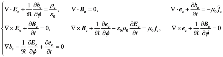
Then, the acoustic equations in (2.10) become a 2-component form

(3.2)

Among which, there are eight equations to be independent

(3.3)

where, is specified by an invariant interval. Correspondingly, the related fields need to be redefined by

(3.4)

with potentials following the Coulomb and Lorenz gauges

(3.5)

By which, an arbitrary potential can be transformed into and. Specifically, for potential, it would require a privileged rest frame, in which the time component can always be set to zero by the gauge transformation. One consequence of (3.3) is that a current with zero divergence (curl) produces no compressive(shearing) field ().

Now, it is easy to calculate two acoustic current stresses (the -component omitted) [6]

(3.6)

with

(3.7)

denote two stress-energy tensors, the Poynting vectors, the corresponding energy densities. Clearly, and both have no contribution to the Poynting’s, implying they are only to achieve the energy conservation through local conversion, rather than radiation. To reinforce the interpretation of, we rewrite the energy flow equations in the form of

(3.8)

The right-hand side of the first (second) equation in (3.8) is a sink (source) term that transfer energy from (to) the acoustic fields to (from) the particles of interacting with the corresponding fields. Specifically, the rate () at which () does work on current () confined to a volume V is called the acoustic Poynting’s theorem;

(3.9)

This desired emphasizes that: the positive (negative) mechanical work done by field () on current () is always equal to the transverse (longitudinal) energy flux through the surface that encloses V subtracting the change rate of the corresponding field energy.

Moreover, the fact of acoustic currents () possessing a dimension of force density (stress/volume) also inspires us to treat them as two drag stresses (). Then, we have the following expressions, including an acoustic source density determined by the drag interaction

(3.10)

It suggests, an acoustic current is always equivalent to a drag force on the surrounding medium, the drag power of. Once such a recognition achieved, we can write (3.3) in the form of

(3.11)

Making use of (3.11) can help us to get the following inhomogeneous wave equations

(3.12)

These equations are more challenging to solve than their homogeneous counterparts, but the introduction of acoustic potentials can help us to get a set of simplified equations

(3.13)

being inhomogeneous equations also, but with much simpler source terms. It is very advantageous for problem-solving that the alternate stress appears on the right-hand sides, which can be used to calculate the acoustic fields produced by dynamically the forced vibration matter system.

If a point time-harmonic acoustic charge with a vibrating amplitude works as a source at the origin, its charge density can be specified by

(3.14)

is the acoustic moment. The continuity equation fixes the associated current density

(3.15)

This current is nothing but a drag force density with transverse and longitudinal components:, by which the acoustic vector potentials are determined as

(3.16)

To use the longitudinal component of (3.16) and integrate the Lorenz gauge condition gives

(3.17)

Which combining with (3.4) can help us to get

(3.18)

as well as the energy flows

(3.19)

Here, is used, denote the angles between position vector and. Accordingly, and read

(3.20)

A striking feature of the obtained above is the coexistence of various terms with different algebraic dependence on the radial distance r from the source. If is the characteristic frequency of harmonic source, we from the second formula of (3.20) find, in the case of low frequency (),can be approximately dominated by

(3.21)

It consists of an oscillating dipole field of, and a proper Coulomb field of. Specifically, the former represents a kind of fluctuation relative to the latter, but no contribution to energy flow. Now, we examine along the direction of, then

(3.22)

This is nothing but a special standing wave with a vibrating amplitude of and wave number k. Importantly, the result reveals the existence of a kind of adjunct waves without contribution to the energy flow, which are characterized by the fields, , so we call them the “adjoint” or “shadow” waves.

By definition, when a compact source radiates its Poynting flow into a differential element of solid angle, it will produce an angular distribution of radiated powers as follows

(3.23)

Correspondingly, the total powers radiated transversely and longitudinally read

(3.24)

which represent the transverse and longitudinal Poynting fluxes through a spherical surface at infinity.

4. The Electromagnetic-Acoustic Equations

4.1. Electromagnetic Equations

As presented by ref [6] , GMEs can directly lead to a longitudinal wave solution, but a very weak radiation. However, no matter how weak, as long as such the radiation could be consented, it is worth studying. So that, we follow (3.3) to rewrite GMEs in 2-component form

(4.1)

with the electromagnetic fields redefined by

(4.2)

followed by the gauge conditions [10]

(4.3)

Correspondingly, the stress on current reads [6]

(4.4)

together with that on

(4.5)

denote two electromagnetic stress-energy tensors, the Poynting vectors, the energy densities. In the case of and, we by (4.1) deduce

(4.6)

Clearly, the equations in first row describe the usual electromagnetic radiation, the remainders the longitudinal and shadow waves. Specifically, although the shadow wave characterized by only works as a fluctuation of Coulomb field and doesn’t contribute to energy flow, we still have a chance to find its whereabouts. For example, an intuitive resonant phenomenon happening between two charged oscillators could help us to achieve our goal (see Figure 1).

To study the electromagnetic properties of matter, we can apply directly the 2-component GMEs (analogous to (3.2)) in a material medium, but need to use two effective electromagnetic interaction ranges instead

of in the corresponding positions. For the time being, would act as two characteristic lengths to de-

termine two modified frequent dispersions, it is tantamount to the transverse and longitudinal photons obtaining their masses. An alternative is to introduce the polarization relations

(4.7)

we get

(4.8)

, are the relative permittivity and permeabilities. To look at the above equations in more detail, an enlightening way is to observe how the electromagnetic fields are related to the potentials and

. It still requires the medium to define its own privileged rest frame, in which the time component. What we call, in this rest frame, the fields are directly from the definitions of (4.2), but need to make an adjustment to the differential operator. So that, we have

(4.9)

4.2. Acoustic Component

Right now, drawing on an analogy with Equation (4.8), we are allowed to apply (3.11) in a macroscopically homogeneous and isotropic unbounded medium with mass density and elastic moduli. This consideration inspires us to reedit the acoustic equations in the form of

(4.10)

followed by

(4.11)

denote the relative mass density and elastic moduli, the propagating speeds of transverse and longitudinal acoustic waves. When (i.e., represent the effective acoustic interaction ranges of elastic medium, analogous to), we have. It suggests and

(4.12)

Then, Equation (4.10) becomes

(4.13)

which, in the case of no driving source, can bring us a set of equations

(4.14)

What the equations describe are very the usual transverse and longitudinal mechanical waves we are familiar with.

Furthermore, we can also express (4.9) and (4.11) in the dualized d’Alembert’s form

(4.15)

with

(4.16)

This unified form would provide us a physical framework to study the electro-acoustic coupling. Table 2 gives a comparison between electromagnetism and acoustics.

5. Detection of Cosmological Acoustic Wave

In electromagnetism, the electric current flowing in conductor is a complex phenomenon, whose microscopic description requires arguments from statistical physics and quantum mechanics. Nevertheless, it is well established phenomenologically that the current density in many systems obeys Ohm’s law: (the electric conductivity). Ohm’s law describes the motion of electrically charged particles (for instance, electrons), which are accelerated by an electric field but suffer energy and momentum degrading collisions with other objects in the system. The linear dependence of on is one consequence of these collisions. If is the average time between collisions, Ohm’s law reads

(5.1)

is the number density of electrons. We here emphasize, the similar situation can also be found in the acoustic system, that is, when an acoustically charged particle with mass m is forced by a field to move with draft velocity in medium, the movement itself is exactly equivalent to an effective force, and thus, there should be. This force together with the collision interaction, can provide us a balance equation

(5.2)

The equality makes it possible for the particle to achieve its acoustic charge

(5.3)

Clearly we see that, the greater mass m and the shorter collision time, the greater acoustic charge. Specifically, if taking the collision time as the cosmological time, the acoustic charge is estimated to be.

Hereby, we borrow Ohm law from electromagnetism and bring it to acoustics. As such, the acoustic Ohm law formally reads

(5.4)

is the acoustic conductivity(analogous to the electric conductivity), the number density of acoustically charge particles.

Importantly, the mechanical explanation of acoustic current allows us to examine the acoustic effect from the perspective of cosmology. To this end, we now recall a full velocity concept [8] , that is defined by the displacement velocity and Hubble velocity as

(5.5)

Following the velocity is the definition of full momentum

(5.6)

The conservation theorem requires

(5.7)

with called the displacement momentum. Such the theorem tell us that, even for a free particle, it will be subjected to an effective damping force, which arises from the collision interaction between the moving particle and virtual pairs, namely

(5.8)

with an average collision time reading the cosmological time. This force in spatial relativity is understood as a spatial relativistic effect [8] , but here it acts as a resistance on the acoustically charged particle at the point. Right now, if notice that, to the resistance, there should be an equal and contrary drag force on CBM

(5.9)

we can find, the acoustic charge of a moving particle is just equal to the product of its mass m and Hubble constant H, namely

(5.10)

identical to the result of (5.3). The result suggests, a mass m at the same time is also an acoustic charge. Therefore, the Coulomb-like force between two rest acoustic charges and can be given by

(5.11)

What it reproduces is nothing but the gravitation, and this identity encourages us to treat the gravitation as a sort of acoustic interaction (see Table 3), the gravitational wave(at least in case of weak fields) as the CAW. Accordingly, the mathematical interpretation of the mechanism of acoustic interaction is naturally provided within the framework of mechanical concepts.

With regard to the CAW, there is a simply designed experiment to detect its presence, by observing the sympathy phenomenon between two simple pendulums (under high vacuum condition). It is shown as Figure 2, a swinging pendulum with mass and cord length, can work as a time-harmonic acoustic moment(defined by (3.14))

(5.12)

is the gravitational acceleration. Then by (3.22), we get the oscillating field along the direction of, that is

(5.13)

In which, the second pendulum (with mass and cord length) will be subjected to a driving force

(5.14)

According to mechanics, this driving force can compel the second pendulum to oscillate, whose oscillating amplitude finally reads

(5.15)

Choosing, , and gives

(5.16)

The result shows, as long as the difference between two cord lengths, the second pendulum will display its observable resonance oscillation. Such oscillation could be seized by Michelson interferometer, notwithstanding the total radiated power of first pendulum only takes an infinitesimal value of

(5.17)

The radiation is so weak that it is extremely difficult to detect.

6. Summary

This work is dedicated to establish a general theoretical framework for the unified description of electromagnetic-acoustic phenomena. In summary we can write:

1) On the stress-energy meaning of the term, we have seen that the cosmological system acts like an elastic medium, such decision allows us to model CAW as a kind of vibration propagating in CBM. The acoustic wave is analogous to the electromagnetic radiation, which follows the Maxwell typical equations, and thus has its own unit-spin quantum in term of phonon. It shows that, besides the transverse and longitudinal radiations, there should be a sort of shadow waves accompanying with them, but no contribution to energy flow.

2) It is suggested that, the electromagnetic-acoustic analogy is a degenerate version of a much deeper one. This deeper version not only provides a consistent approach to examine synthetically the general properties of electromagnetic and acoustic motions, but also can help us to study the intrinsic mechanism of electro-acoustic coupling in physics.

3) The acoustic charge carried by a moving particle has been verified to be proportional to its mass with a scale coefficient of Hubble constant, by which the determined acoustic interaction is just equal to the gravitational force. Therefore, the decision allows us to understand the gravitational interaction as the acoustic interaction, and the gravitational wave as CAW. Finally, the feasibility of measuring this acoustic wave (referring to its shadow component) is discussed.

Cite this paper

Qiankai Yao, (2016) A Deeper Analogy between Electromagnetism and Acoustics. Open Access Library Journal,03,1-16. doi: 10.4236/oalib.1102280

References

- 1. Lafarge, D. and Nemati, N. (2013) Nonlocal Maxwellian Theory of Sound Propagation in Fluid-Saturated Rigid-Framed Porous Media. Wave Motion, 50, 1016-1035.
http://dx.doi.org/10.1016/j.wavemoti.2013.04.007 - 2. Russakoff, G. (1970) A Derivation of the Macroscopic Maxwell Equations. American Journal of Physics, 38, 1188.
http://dx.doi.org/10.1119/1.1976000 - 3. Landau, L.D. and Lifshitz, E. (1960) Electrodynamics of Continuous Media. Pergamon Press, Oxford.
- 4. Schoch, A. (1953) Remarks on the Concept of Acoustic Energy. Acustica, 3, 181.
- 5. Berestetskii, V.B., et al. (1980) Quantum Electrodynamics. 2nd Edition, Pergamon, Oxford.
- 6. Yao, Q.K. (2015) The Unified Theoretical Form of Massive Electrodynamics. Open Access Library Journal, 2, e1372.
http://dx.doi.org/10.4236/oalib.1101732 - 7. Peebles, P.J.E. (1993) Principles of Physical Cosmology. Princeton University Press, Princeton.
- 8. Yao, Q.K. (2015) The Spatial Relativity and Its Physical Consequences. Open Access Library Journal, 2, e1286.
http://dx.doi.org/10.4236/oalib.1101286 - 9. Yao, Q.K. (2015) Magnetic Monopole Cannot Be Incorporated into the Dual Framework of Electromagnetic Theory. Open Access Library Journal, 2, e1955.
http://dx.doi.org/10.4236/oalib.1101955 - 10. Zangwill, A. (2012) Modern Electrodynamics. Cambridge University Press, Cambridge.