Received 18 February 2015; accepted 6 March 2015; published 10 March 2015

ABSTRACT

This study employs the Fireman Method in the solutions of optimal control problems of the form, under an admi- ssible control, which causes to follow admissible trajectory. The Hamiltonian Principle was employed for the analytical solutions of the given optimal control problems. It has been observed that this method converges close to the analytical solution for some class of problems.

Keywords:

Fireman Method, Optimal Control, Hamiltonian Principle, Linear Quadratic Regulator

Subject Areas: Mathematical Analysis, Mathematical Statistics, Operational Research

1. Introduction

A well known approach to the principle of optimization was first scribbled centuries ago on the walls of an ancient Roman bathhouse in connection with a choice between two aspirants for emperorship of Rome. Out of two evils, we always choose the lesser. In everyday life, decisions are made to accomplish certain tasks. Normally, there exist several possible ways or methods by which a certain task can be accomplished. Some of these methods may be more efficient or reliable than others and the presence of physical constraints implies that, not just any method can be used. It thus becomes necessary to consciously determine the “best” or “optimal” way to accomplish the task [1] .

Optimization is the act of obtaining the best policies to satisfy certain objectives while at the same time satisfying some fixed requirements or constraints. It involves the study of optimality criteria for problems, the determination of algorithmic methods of solution, the study of the structure of such methods and computer implementation of the methods under both trial conditions and real life problems [2] .

According to Wikipedia, optimization can be defined as a process of finding an alternative with the most costeffective or highest achievable performance under given constraints, by maximizing desired factors and minimizing undesired ones. In comparison, maximization means trying to attain the highest or maximum result or outcome without regard to cost or expense. The Practice of optimization is restricted by lack of full information and lack of time to evaluate available information. In computer simulation (modeling) of business problems, optimization is achieved usually by usinglinear programming techniques of operations research.

Optimization takes its root from the word optimizes, which is to make as perfect, effective, or functional as possible. In engineering, optimization is a collection of methods and techniques to design and make use of engineering systems as perfectly as possible with respect to specific parameters. In industrial engineering, one typical optimization problem is in inventory control. For this problem, we want to reduce the costs associated with item stocking and handling in a warehouse. In the simplest form of this problem, the parameters to be optimized are the quantity of inventory required to fill existing and anticipated orders, when that inventory has to be available and the physical capacity of the warehouse. Optimization requires the representation of the problem in a mathematical model where the decision variables are the parameters of the problem [3] .

Optimization is an act of finding an alternative with the most cost effective of highest achieveable perfor- mances under the given constraints by a maximizing desire factors and minimizing undesire ones. In comparison, maximization means trying to attain the highest of mininum result or outcome without regard to cost or expense. Practice of optimization is restricted by the lack of full information and the lack of time to evaluate what information is available. The essence of an optimization problem is like catching a black cat in a dark room in minimal time. (A constrained optimization problem corresponds to such a roomful of furniture). A light, even dim, is needed. Hence optimization methods explore assumptions about the character of response of the goal function to varying parameters and suggest the best way to change them. The variety of a priori assumptions corresponds to the variety of optimization methods [4] .

Optimization is a process, or methodology of making something (as a design, system, or decision) as fully perfect, functional, or effective as possible; specifically: the mathematical procedures (as finding the maximum of a function) involved in this [5] .

1.1. Optimal Control

In many areas of the empirical sciences such as Mathematics, Physics, Biology, and Chemistry, as well as in Economics, we study the time development of systems. Certain essential properties or characteristics of the system, called the state of the system, change over time. If there are n state variables we denote them by The rate of change of the state variables with respect to time is usually subject to an error. This is due to many factors, including the actual values of the and on certain parameters that can be controlled from the outside. These parameters are called control variables and are denoted by. We shall assume throughout this work that the laws governing the behavior of the system over time are given by systems of ordinary differential equations. The control variables can be freely chosen within certain bounds. If the system is in some state x⁰ at time, t₀, and if we choose a certain control function u(t), then the system of differential equations will, usually, have a unique solution, x(t). If there are a priori bounds on the values of the state variables, only those control functions will be admissible which give rise to state functions x(t) satisfying the bounds. In general, there will be many admissible control functions, each giving rise to a specific evolution of the system. In an optimal control problem, an optimality criterion is given which assigns a certain number (a “utility”) to each evolution of the system. The problem is then to find an admissible control function which minimizes the optimality criterion in the class of all admissible control functions. The tools available for solving optimal control problems are analogous to those used in static optimization theory. Before examining a simple control problem, let us digress a little with some remarks concerning static optimization [6] .

1.2. Problem Formulation

The axiom “A problem well put is a problem half solved” may be a slight exaggeration, but its intent is nonetheless appropriate. In this paper, we shall discuss the important aspects of problem formulation. The formulation of an optimal control problem requires:

1. A mathematical description (model) of the process to be controlled.

2. A statement of the physical constraints.

3. Specification of a performance criterion.

A nontrivial part of any control problem is modeling the process. The objective is to obtain the simplest mathematical description that adequately predicts the response of the physical system to all anticipated inputs. Our discussion will be restricted to systems described by ordinary differential equations (in state variable form). Thus, if

are the state variables ( or simply the states ) of the process at time t, and

are the control inputs to the process at time t, then the system may be described by n first-order differential equations

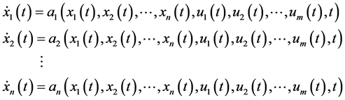
We can define as the state vector of the system, and 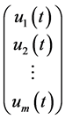as the control vector. The state equations can then be written as:

where [7] .

History of control input values during the interval is denoted by u(t) and is called a control history or simply a control. Also, history of state values in the interval is called a state trajectory and is denoted

by x(t). However, we have to note that the terms “history”, “curve”, “function”, and “trajectory” are used interchangeably [8] .

1.3. A Sketch of the Problem

Let us begin with a rough sketch of the type of economic problems that can be formulated as optimal control problems. In the process we introduce our notation. An economy involving time can be described by n real numbers

(1.3.1)

The amounts of capital goods in n different sectors of the economy might, for example, be suitable state variables. It is often convenient to consider (1.3.1) as defining the coordinates of the vector in. As t varies, this vector occupies different positions in, and we say that the system moves along a curve in, or traces a path in. Let us assume now that the process going on in the economy (causing the’s to vary with t) can be controlled to a certain extent in the sense that there are a number of control functions

(1.3.2)

that influence the process. These control functions, or control variables, also called decision variables or instruments will typically be economic data such as tax rates, interest rates, the allocations of investments to different sectors etc. [9] .

To proceed we have to know the laws governing the behavior of the economy over time, in other words the dynamics of the system. We shall concentrate on the study of systems in which the development is determined by a system of differential equation in the form

(1.3.3)

The functions are given functions describing the dynamics of the economy. The assumption is thus that the rate of change of each state variable, in general, depends on all the state variables, all the control variables, and also explicitly on time t. The explicit dependence of the functions on t is necessary, for example, to allow for the laws underlying (8) to vary over time due to exogenous factors such as technological progress, growth in population, etc.

By using vector notation the system (1.3.3) can be described in a simple form. If we put

then (1.3.3) is equivalent to

(1.3.4)

Suppose that the state of the system is known at time so that, where is a given vector in. If we choose a certain control function defined for and insert it into (1.3.3), we obtain a system of first-order differential equations with n unknown functions.

Since the initial point is given, the system (1.3.3) will, in general, have a unique solution

. Since this solution is “a response” to the control function u(t), it would have been appropriate to denote it by but we usually drop the subscript u.

By suitable choices of the control function u(t) many different evolutions of the economy can be achieved. However, it is unlikely that the possible evolutions will be equally desirable. We assume, then, as is usual in economic analysis, that the different alternative developments give different “utilities” that can be measured. More specifically, we shall associate with each control function and its response the number

(1.3.5)

where is a given function. Here is not necessarily fixed, and might have some terminal condition on it at the end point. The fundamental problem that we study in this chapter can now be formulated:

Among all control functions u(t) that via (1.3.4) bring the system from the initial state to a final state satisfying the terminal conditions, find one (provided there exists any) such that J given by (1.3.5) is as large as possible. Such a control function is called an optimal control and the associated path x(t) is called an optimal path. is often called the criterion functional.

1.4. Motivation for the Study

The study was motivated by the fact that the method used followed sequential order: the Hamiltonian “” was derived from the combination of the state equation (which depends on the admissible control) and the performance measure; the co-state and the state variables could be obtained from the solutions of ordinary differential equations of the co-state and state equations respectively. Also, an admissible control which causes to follow admissible trajectory that minimizes the performance measure could be determined. In addition, the results compared considerably with the computer implementation results.

1.5. Statement of the Problem

The problem statements are stated as follows:

Is it possible to find among all control functions which bring x(t) from the initial point to a point satisfying the given terminal condition, one which makes the integral in (1.3.5) as small as possible (provided such a control function exists)?

Is any correlation exists between Fireman method and computer implementation method in the solutions to this class of problems?

2. Nature of Optimal Control

The task in static optimization is to find a single value for each choice variable, such that a stated objective function will be maximized or minimized as the case maybe. Such a problem is devoid of a time dimension. In contrast, time enters explicitly and prominently in a dynamic optimization problem. In such a problem, we will always have in mind a planning period, say, from an initial time t = 0 to a terminal time t = T, and try to find the best course of action to take during that entire period. Thus the solution for any variable will take the form of not a single value, but a complete time path. Alpha discusses further that, suppose the problem is one of profit maximization over a time period. At any point of time, we have to choose the value of some control variable, u(t), which will then affect the value of some state variables y(t), via a so-called equation of motion. In turn y(t) will determine the profit. Since the objective is to maximize the profit over the entire period, the objective function should take the form of a definite integral of from t = 0 to t = T. To be complete, the problem also specifies the initial value of the state variable, and the terminal value of y, y(T) or alternatively, the range of value that y(T) is allowed to take. Taking into account of preceding, one can state the simplest problem of optimal control as

Maximize

Subject to

, free and for all

The first line of the objective function is an integral whose integral f(t, y, u) stipulates home the choice of the control variable u at time t, along with the resulting y at time g, determines our object of maximization at time t. The second is the equation of the motion for the state variable y. What this equation does is to provide the mechanism whereby our choice of control variable u can be translated into a specific pattern of, movement of the state variable y can be adequately described by a first-order differential equation, then, there is need to transform this equation into a pair of first-order differential equations. In this case an additional state variable will be introduced [10] .

2.1. Linear Quadratic Control

A special case of a general non-linear optimal control problem is the linear quadratic (LQ) optimal control problem. Linear quadratic problem is given as follows;

Minimize the quadratic continuous-time cost functional

(2.1.1)

Subject to the linear first-order dynamic constraints

(2.1.2)

and the initial condition [11] .

A particular LQ problem that arises in many control system problem is that of the linear quadratic regulator (LQR) where all of the matrices (i.e. A, B, Q and R) are constants, the initial time is arbitrarily set to zero, and the terminal time is taken as the (the last assumption is what is known as infinite horizon).

Furthermore, the LQR problem is stated as follows: Minimize the infinite horizon quadratic continuous-time cost function

(2.1.3)

subject to the linear time-invariant first order dynamic constraints, and initial condition.

In the finite-Horizon case, the matrices are restricted in the Q and R are positive semi-definite and positive definite and in the infinite horizon case, however the matrices Q and R are not only semi-definite and positive respectively, but are also constants [12] .

2.2. Linear-Quadratic Regulator

The theory of optimal control is concerned with operating dynamical systems at minimum cost. The case where the system dynamics are described by a set of linear differential equations and the cost is described by a quadratic functional is called the LQ problem. One of the main results in the theory is that the solution is provided by the Linear-Quadratic Regulator (LQR), a feedback controller whose equations are given in Section 2.3. [13] .

General Description of Linear Quadratic Regulator

In layman’s terms this means that the settings of a (regulating) controller governing either a machine or process (like an airplane or chemical reactor) are found by using a mathematical algorithm that minimizes a cost function with weighting factors supplied by a human (engineer). The “cost” (function) is often defined as a sum of the deviations of key measurements from their desired values. In effect this algorithm finds those controller settings that minimize the undesired deviations, like deviations from desired altitude or process temperature. Often the magnitude of the control action itself is included in this sum so as to keep the energy expended by the control action itself limited.

In effect, the LQR algorithm takes care of the tedious work done by the control systems engineer in optimizing the controller. However, the engineer still needs to specify the weighting factors and compare the results with the specified design goals. Often this means that controller synthesis will still be an iterative process where the engineer judges the produced “optimal” controllers through simulation and then adjusts the weighting factors to get a controller more in line with the specified design goals.

The LQR algorithm is, at its core, just an automated way of finding an appropriate state-feedback controller. As such it is not uncommon to find that control engineers prefer alternative methods like full state feedback (also known as pole placement) to find a controller over the use of the LQR algorithm. With these the engineer has a much clearer linkage between adjusted parameters and the resulting changes in controller behavior. Difficulty in finding the right weighting factors limits the application of the LQR based controller synthesis.

2.3. Finite-Horizon, Continuous-Time LQR

For a continuous-time linear system, defined on, described by

(2.3.1)

with a quadratic cost function defined as:

(2.3.2)

The feedback control law that minimizes the value of the cost is

(2.3.3)

where is given by

(2.3.4)

and is found by solving the continuous time Riccati differential equation.

(2.3.5)

The first order conditions for J_min are

(i). State equation

(2.3.6)

(ii). Co-state equation

(2.3.7)

(iii). Stationary equation

(2.3.8)

(iv). Boundary conditions

(2.3.9)

2.4. Review of Linear Ordinary Differential Equation

Optimal control involves among other things, the ordinary differential equations. Hence, this work deems it necessary to consider the state equation together with the solution of the ordinary differential equation. The solution of an ordinary differential equation (ODE) is given by

Let be the unique solution of the matrix ODE

(2.4.1)

We call, a fundamental solution, and sometimes write

(2.4.2)

the last formula being the definition of the exponential. Observe that:

(2.4.3)

The theorem for solving linear system of ODE as follows.

Theorem 2.4.1

(i) The unique solution of the homogeneous system of ODE

(2.4.4)

is

(ii) The unique solution of the non-homogeneous system

(2.4.5)

is (2.4.6)

And that this expression is the variation of parameters formula [14] .

3. The Algorithmic Frame Work of Continuous Linear Regulator Problems

In this section, we shall now proceed to the steps involved in the algorithmic frame work of linear regulator problems:

Step 1: There is need for noting the coefficient of the state equation (s):

where and are the state and control functions respectively, and A and B are constants. If there is one state equation, we then demand for the values of A₁ and B₁.

Step2: The initial boundary condition(s). For one state equation, we demand ₁x₀, and ₁t₀.

Step3: The coefficient of the performance measure to be minimizes (or maximizes)

where is the integral lower limit, is the integral upper limit, and are constant matrices.

Step 4: The Lagrangian is given by

Step 5: We find the co-state equation. For one state equation, derivative of l, i.e.

Step 6: Derive the optimally condition from the Lagrangian. For one state equation, we find

Step7: We determine the boundary condition with

Step 8: The next is to enter the initial guess value for the optimal control

Step 9: Integrate the state equation, substituting the control initial guess

value i.e. standard integral gives

,

If is a constant. Otherwise, we have

Optimal Control and Hamiltonian

The objective of optimal control theory is to determine the control signals that will cause a process to satisfy the physical constraint and at the same time minimizes (or maximizes) some performance measures. The state of a system is a set of quantities which if known at are determined for by specifying the inputs to the system for. It is worthy to state the various components of maximum principle for problem of the form

Subject to

is free and as follows:

(i)

(ii) (State equation)

(iii) (Co-state equation)

(iv) (Transversality condition)

Condition (i) states that at every time, the value of, the optimal control , must be chosen so as to maximizes the value of the Hamiltonian over all admissible value of. In case the Hamiltonian is differen-

tiable with respect to and yields an interior solution, condition: i) can be replaced by. However, if the control region is a closed set, then boundary solutions are possible and may not apply. In fact the maximum principle does not ever required the Hamiltonian to be differentiable with respect to. Conditions ii) and iii) of the maximum principle and give us two equations of motion referred to as the Hamiltonian system for the given problem. Condition iv), is the transversality condition appropriate

for the free-terminal-state problem only. It is noted that, for optimal control problem, the Lagrange function and the Lagrange multiplier variable are known as the Hamiltonian function and co-state variable. The co-state variable measures the shadow price of the state variable [15] .

4. Fireman Numerical Method for a Class of Existing Optimal Control Problems

This self developed method made use of the application of Geometric Progression and Hamiltonian method to numerical solution of some existing Optimal Control Problems of the form “Find an admissible control which causes to follow admissible trajectory that minimizes:

(4.1)

where”.

Theorem 4.1.

For the initial control and step length, the control update is given as:

(4.2)

Proof

Let be the initial control for the system (4.1), then the successive control updates are given as:

(4.3)

Continuing this way, we have that

Theorem 4.2.

The solution of the state equation in (4.1) is given as:

where

Theorem 4.3.

The solution of the state is given as

as

Theorem 4.4: The algebraic relationship is given as:

4.1. Algorithmic Framework of Fireman Method

1. Find the Hamiltonian: The Hamiltonian is given by

2. Determine the Optimality condition from the Hamiltonian:

3. Obtain and solve the co-state equation

4. Update the control using 0.1 as step length:

5. Find the update of the state:

where

6. Obtain the algebraic relationship:

7. Test for optimality:

8. Test for convergence with:

4.2. Test Problem

In this problem, we consider a non-economic problem. This is finding the shortest path from a given point A to a given straight line. In the diagram below, point A have been plotted on the vertical axis in the t-x plane, and drawn the straight line as vertical one at. Three out of an infinite numbers of admissible paths are also shown, each with a different length. The length of any path is the aggregate of small paths segments, each of which can be considered as the hypotenuse of a triangle (may not be drawn) formed by small movements dt and dx.

By Pythagoras’ theorem, we denote the hypotenuse by

(4.2.1)

Leading to

(4.2.2)

by simple calculations on division by dt²

Let, so that

(4.2.3)

The total length of the path can then be found by integrating (4.2.3) with respect to from to. If we let be the control variable, then (4.2.3) can be expressed as:

(4.2.4)

The shortest path problem is to find an admissible control, which causes to follow admissible trajectory that minimizes

(4.2.5)

Solution to (4.2.5) is same as that of minimization i.e.

Minimize (using distance problem)

Subject to

(4.2.6)

and

4.3. Analytical Solution to Problem

The problem is same as that of

Max.

Subject to

(4.3.1)

and

The Hamiltonian for the problem is given by

Since ℋ is differentiable in, and is unrestricted, the following first order condition can be used to maximize ℋ.

Making the subject of relation, we have that.

Checking the second order condition we find.

This result verifies that the solution to does maximize the Hamiltonian. Since is a function of l, we need a solution to the co-state variable. From the first order conditions the equation of motion for the co-state variable is

Integrating, we have, where is a constant.

Since is independent of, we have that l is a constant. To definitive this constant we can make use of the transversality condition,. Since can take only a single value now known to be zero, we ac-

tually have . Thus we can write .

It follows that the optimal control is. In addition, if we use the equation of motion for the state variable, we see that or (which is a constant). Thus we may write . Since, then the shortest path from a given point A to a given straight line with zero gradient.

4.4. Results of the Test Problem

Analytic:

Table of Results for Problem

5. Summary

It has been established that the knowledge of the Hamiltonian method and the computer programming method has made the minimization (or maximization) process possible for optimal control problems of the types considered above. The two methods in addition to the solution of differential equations involved made the solutions possible. One of the advantages of Fireman method is that, it compared considerably with the computer implementation results.

5.1. Conclusions

This paper has revealed that mathematics should not be studied in abstraction. There is reality in mathematics. The practical and real life situations should be the main focus of mathematics, like distances, consumption problems etc. The co-state, control variable, associated with optimal control problem coupled with a system of linear dynamic constraints solved by Hamiltonian method, have been found to be a very powerful mathematical tool with numerous applications.

More so, computationally, the Fireman Method was tested on an existing linear-quadratic regulator problem with the result obtained. Our numerical and analytic results for this problem are presented in the table below, with the summary as:

Based on the results, it is obvious that, on determining the optimal controls and trajectories of linear-quadratic regulator problems using iterative numerical technique such as Fireman Method is relevant and recommended for use. It is observed that results obtained from Fireman method are much closed to the numerical result and have higher rate of convergence.

5.2. Recommendation

It is recommended that further researches should be carried out on the application of penalty function method to minimize (or maximize) the tested problems and other problems still in existence. One could consider the use of the steepest descent method.

Cite this paper

J. O. Olademo,A. A. Ganiyu,M. F. Akimuyise, (2015) Fireman Numerical Solution of Some Existing Optimal Control Problems. Open Access Library Journal,02,1-14. doi: 10.4236/oalib.1101352

References

- 1. Thomas, D. (2001) Optimization Method of Control Processes with Minimis Criteria iii, Automat, (i).Tekmekhem.
- 2. Mital, K.V. (1976) On Program Pursuit Problems in Linear System. Izvestia Aced, Nauk, Automat, (i).Tekmekhem.
- 3. Kirk, D.E. (2004) Optimal Control Theory (An Introduction). Dover Publications, INC. Mineola, New York.
- 4. Seiersted, A. and Sydsaeter, K. (1985) Optimal Control Theory with Economic Application. Amsterdem, Lansame Publisher, New York.
- 5. Snyman, J.A. (2005) Practical Mathematical Optimization. Springer, USA.
- 6. Sontag, E.D. (1998) Mathematical Control Theory: Deterministic Finite Dimensional Systems. 2nd Edition, Springer, Berlin.
http://dx.doi.org/10.1007/978-1-4612-0577-7 - 7. Hull, D.G. (2003) Optimal Control Theory for Applications. Springer-Verlag Inc., New York.
- 8. Gurman, V.I. and Krotov, V.F. (1973) Methods and Problems of Optimal Control. Nauka, Moskva.
- 9. Todorov, E. (2006) Optlmal Control Theory. MIT Press, Cambridge.
- 10. Alpha, C.C. and Kelvin, W. (2005) Fundamental Methods of Mathematical Economics. McGraw-Hill Companies, New York.
- 11. Rose, M. (2009) Theory and Methods of Projecting Automati Controllers. Automat I, Telemakhan, N.I.
- 12. Bertsekas, D.P. (2012) Dynamic Programming and Optimal Control. Standard University, Standard.
- 13. Subbotin, A.I. and Krasovskii, N.N. (1988) Game-Theoretical Control Problems. Springer-Verlag, New York.
- 14. Evans, L.C. (2001) An Introduction to Mathematical Optimal Control Theory, Versiono. L.
http://math.berkeley.edu/’evans/sde - 15. Krotov, V.F. (1996) Global Methods in Optimal Control Theory. Mercel Dekker, Inc., New-York.