Open Access Library Journal
Vol.02 No.01(2015), Article ID:67994,14 pages
10.4236/oalib.1100745
Analysis of EEG Dynamics in Epileptic Patients and Healthy Subjects Using Hilbert Transform Scatter Plots
Chandrakar Kamath
Ex. Professor, Electronics and Communication Department, Manipal Institute of Technology, Manipal, India
Email: chandrakar.kamath@gmail.com
Copyright © 2015 by author and OALib.
This work is licensed under the Creative Commons Attribution International License (CC BY).
http://creativecommons.org/licenses/by/4.0/


Received 27 December 2014; accepted 16 January 2015; published 22 January 2015
ABSTRACT
In this study, we investigated the electroencephalogram (EEG) dynamics in normal and epileptic subjects using three newly defined quantifiers adapted from nonlinear dynamics and Hilbert transform scatter plots (HTSPs): dispersion entropy (DispEntropy), dispersion complexity (Disp Comp), and forbidden count (FC), hypothesizing that analysis of electroencephalogram (EEG) signals using nonlinear and deterministic chaos theory may provide clinicians with information for medical diagnosis and assessment of the applied therapy. DispEntropy evaluates irregularity of the EEG time series. DispComp and FC quantify degree of variability of the time series. Receiver operating characteristic (ROC) analysis reveals that all the three quantifiers can discriminate between seizure and non-seizure states with very high accuracy. The application of such a technique is justified by ascertaining the presence of nonlinearity in the EEG time series through the use of surrogate test. The false positive rejection of the null hypothesis is eliminated by employing Welch window before the computation of the Fourier transform and randomizing the phases, in the generation of the surrogate data. Paired t-test revealed significant differences between the measures of the original time series and those of their respective surrogated time series, indicating the pre- sence of deterministic chaos in the original EEG time series.
Keywords:
Deterministic Chaos, Electroencephalogram, Epilepsy, Hilbert Transform Scatter Plot, Nonlinear Analysis, Surrogate Data Test
Subject Areas: Bioengineering, Neuroscience

1. Introduction
Epilepsy is one of the world’s most common chronic neurological disorders, which is characterized by paroxysmal and hyper-synchronous activity of the neurons in the cerebral cortex leading to recurrent and unpredictable interruptions of normal brain function, called epileptic seizures [1] . The symptoms depend upon the location of the seizure onset in the brain and the spread of the seizure. In most patients the seizures occur suddenly without any identifiable precipitants. This unpredictable nature of epilepsy is a major threat in patients with uncontrolled epilepsy. Detection of seizure onset, even in the short-term, would provide time to take preventive measures to keep the risk of seizure to a minimum and ultimately improve quality of life. Since epilepsy is a condition related to electrical activity of the brain, the electroencephalogram (EEG) signal is the most widely accepted clinical tool for the evaluation, diagnosis and treatment of epilepsy. Long-term EEG monitoring can provide about 90% diagnostic information and thus becomes a gold standard in epilepsy diagnosis [2] . However, even for at rained neurologist the detection of seizures can be challenging as well as time-consuming from visual inspection of EEG for different reasons such as excessive presence of myogenic artefacts [3] . Hence, several methods have been proposed to automatically detect epileptic seizures by analyzing EEG data. One of the most explored topics in nonlinear EEG analysis today is epilepsy. Epileptic brain, like other nonlinear chaotic system repeatedly, but intermittently, makes abrupt transitions into and out of the seizure state [4] - [9] . The behavior has been attributed to the epileptogenic focus driving the brain into self-organizing phase transitions from chaos to order. The EEG correlate of such a transition is characterized by the abrupt appearance of well organized oscillations out of the ongoing background activity, a characteristic of a seizure. In the waking state, the ongoing background activity is described by low to medium amplitude electrical activity, dominated by irregular waveforms. During seizure, this background activity is replaced by rhythmic, higher amplitude, organized, and self- sustained signal. In fact, the reverse transition (resetting mechanism) from order to chaos is initiated by the occurrence of a seizure [10] . This dualism of chaos and order is the key feature of nonlinear dynamics. Since EEG signal may be considered chaotic, deterministic chaos theory seems to be promising to study the EEG dynamics and the underlying chaos in the brain [11] . It has been shown in the literature that nonlinear analysis permits an improvised characterization and relative comparison of different physiological/pathological brain states [12] [13] . More importantly, nonlinear methods may be applied to linear signals, but the vice-versa is not true. Various nonlinear, entropy, and complexity algorithms have been developed and tried in the past two decades to characterize chaotic behavior in the EEG time series [14] - [22] . Further, the recent advances in the area of chaos and nonlinear dynamics analysis have revealed fractal patterns and chaotic properties of natural phenomena leading to a shift in the paradigm. A strong reason for this paradigm shift is the acknowledgement of variability in natural systems to be healthy, and in fact, is desirable. Such variability allows accommodating external perturbations [23] . It is also found that use of standard chaotic quantifiers, like correlation dimension and Lyapunov exponents, demand long stationary electroencephalogram (EEG) epochs and long processing time [24] [25] . Further, when these quantifiers were computed over EEG epochs before and after therapy, they did not show a proper discrimination in the EEG states [25] . Hence, there was a need for the usage of other quantifiers. It is also found that the irregularity and degree of variability of the EEG time series change depending on the physiological/pathological brain state and we proposed measures for irregularity and rate of change of variability, each of which can serve as a stand-alone indicator for medical diagnosis. In this pilot study, we investigate the EEG background dynamic activity in normal and epileptic subjects using three newly defined quantifiers adapted from Hilbert transform scatter plot (HTSP), namely dispersion entropy (DispEntropy), dispersion complexity (DispComp), and forbidden count (FC). All the measures can detect changes in EEG characteristics (dynamics) and discriminate epileptiform epochs from interictal events and eye blinks. The prime advantages of these quantifiers are: 1) they can be used to characterize a signal irrespective of the nature of the underlying dynamics, i.e. whether the signal is chaotic, deterministic, or stochastic. 2) The mean value of these quantifiers changes significantly before, during, and after seizures. This almost eliminates the requirement of thresholds to determine onset and offset of seizure. 3) DispComp and FC have the advantage of very easy implementation and fast computation.
2. Methods and Materials
2.1. EEG Data
In this study, we use two sets of databases. The first is the Bonn University EEG database [26] and the second database is the CHB-MIT scalp database (chbmit) of Physionet [27] , both freely available in public domain. The Bonn EEG data, described by Andrzejak et al. [26] , is from three different groups: normal, inter-ictal and ictal and is categorized into five sets (designated A-E), each containing 100 single channel EEG segments of 23.6 s duration, sampled at 173.6 samples per sec with 12 bit resolution. Each data segment has 4096 samples. The bandpass filter setting was at 0.53 - 40 Hz (12 dB/octave). Each set was recorded under different conditions. These segments have been picked from continuous multi-channel EEG recordings after removal of any artifacts, like, muscle activity, or eye movements, making sure that they fulfilled stationarity requirements. Each segment is treated as a separate EEG signal so that in all there are 500 EEGs. All the EEG signals were recorded using the same 128-channel amplifier system using an average common reference. This large data set improves statistical significance during comparison of results. Sets A and B contain segments taken from surface EEG recordings acquired from five healthy volunteers using a standard 10 - 20 electrode placement scheme. The subjects were awake and relaxed with their eyes open for set A and eyes closed for set B, respectively. The segments for sets C, D, and E were acquired from five epileptic patients undergoing presurgical diagnosis. The diagnosis was temporal lobe epilepsy (epileptogenic focus: hippocampal formation). Sets C and D contained only activity measured during seizure free intervals (interictal epileptiform activity), with segments in set C recorded from hippocampal formation of the opposite hemisphere of the brain and those in set D recorded within epileptogenic zone. On the other hand, set E contained only seizure activity (ictal intervals), with all segments recorded from sites exhibiting ictal activity.
The CHB-MIT scalp database includes recordings from 22 pediatric epileptic patients with intractable seizures (males:  and age = 3 - 22 years; females:
  and age = 1.5 - 19 years). The surface recordings were of approximately 6 hours duration per patient, each with 182 seizures and sampled at 256 Hz.
The robustness of DispEntropy, DispComp, and FCin discriminating different EEG states was first investigated on Bonn Database, which included all the five sets A-E, each with 100 single channel EEG segments of 23.6 s duration. We also explored the diagnostic ability of these three quantifiers on a randomly selected EEG signal from CHB-MIT database and compared the performance with other two popular quantifiers used in nonlinear analysis. To our knowledge, there is no study in the literature related to DispEntropy, DispComp, and FCHTSP analysis for epilepsy seizure detection. The obtained results indicate high accuracy.
2.2. Hilbert Transform (HT)
Hilbert transform (HT) has been extensively used in the analysis of nonlinear signals. The HT is a time-domain to time-domain transformation which shifts the phase of a signal by 90 degrees. In the process the positive frequency components in the signal are shifted by +90 degrees, and negative frequency components are shifted by −90 degrees. Though the Hilbert transform like the fast Fourier transform (FFT) is a linear operator, it is useful for analyzing nonstationary signals by expressing frequency as a rate of change in phase, so that the frequency can vary with time. The HT and FFT give the same results when both transforms are applied to signals having the relatively long durations needed for the FFT and wavelets [28] [29] . Otherwise they are complementary.
If  represents a real signal, it is possible to construct a complex valued signal
 , called analytic signal of
 , such that
 , where
  is the Hilbert transform of
 . The Hilbert transform of a signal
  is defined as the convolution of
  with
with  as given by the following equation.
 (1)
(1)
where the integral is to be interpreted as a Cauchy principal value. This convolution can be thought of as a filtering operation with a quadrature filter which shifts all sinusoidal components by a phase shift of . Using Fourier identities, the Fourier transform of
  is given by
 (2)
(2)
 (3)
(3)
In the frequency domain, the result is then obtained by multiplying the spectrum of ,
,  , by
, by 
 for negative frequencies and
  (90) for positive frequencies. The time domain result can then be obtained performing an inverse Fourier transform. This means that the Hilbert transform of the original signal
  represents its harmonic conjugate. It is to be noted that the amplitudes of the Fourier transforms of
  and of
  are identical, they differ only in phase. In this study, HT is used as a phase shifter and the Hilbert transformed signal is used in a scatter plot.
2.3. Hilbert Transform Scatter Plot (HTSP)
A Poincare plot is a nonlinear method with an ability to capture the nonlinear pattern of the system dynamics [30] . A standard Poincare plot, a scatter plot where a time series  is plotted against its delayed version
 , delayed by 1 sample. A lagged Poincare plot, an extended version of the standard Poincare plot, a scatter plot where a time series
  is plotted against its delayed version
 , delayed by
  samples. On the other hand, a graph of
  plotted against
  produces a scatter plot of first differences of the data, which is called a second-order difference (SOD) plot of
  [31] . In this work, we develop a scatter plot by plotting the EEG time series under investigation against its Hilbert transform, which we call Hilbert transform scatter plot (HTSP). Since the Hilbert transformed signal is a phase shifted version of the original signal, it is obvious that HTSP is a lagged Poincare plot. Unlike a Poincare plot which is usually confined to first quadrant of the coordinating system, a HTSP which is centered about the origin like SOD plot, can be useful tool to physicians, who can make a preliminary diagnosis by the visual inspection of these scatter diagrams. SOD has been found to be useful in the study of chaotic systems, like hemodynamic systems and in classification problems, like separating congestive heart failure patients from normal subjects [31] - [34] . The most commonly used measure in conjunction with SOD plot is the central tendency measure (CTM), which quantifies the degree of variability in a scatter plot. In this study, however, we define dispersion entropy, dispersion complexity, and forbidden count, all derived from HTSP, to estimate the irregularity, complexity or degree of variability in the HTSP.
2.4. Dispersion Entropy (DispEntropy), Dispersion Complexity (DispComp), and Forbidden Count (FC) in the Context of HTSP
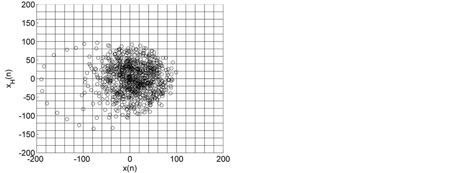
In this study, we divide the HTSP spatial coordinate system into a matrix of elements using an M × M grid ordered from top to bottom and left to right, so as to accommodate the most extreme point in the scatter plot, as shown in Figure 1. Each cell represents a subspace in the HTSP space. For example, the bottom-left cell extends over the range  and
and ; the top-left cell extends over the range
  and
and ; the top-right cell extends over the range
  and
and ; and the bottom-right cell extends over the range
  and
and . The HTSP in the figure has 1200 × 1200 = 1,440,000 cells which constitutes total count of the matrix. We first mark all the points in the HTSP scatter space and count the number of points in each cell. Next, we convert this matrix figure into an image, treating the cells as if they were pixels and with the point counts in the cells corresponding to the intensity of the pixels in the image. Then we find the entropy of this gray scale image. To accomplish this we adopt the following steps: 1) We compute the histogram of the distribution of the counts in the matrix, with the dynamic range of the data being transformed to fit into gray scale range; 2) From the histogram we find the probability distribution of the bins in the histogram; 3) We then apply Shannon’s entropy to the probability distribution. The resulting entropy constitutes dispersion entropy (DispEntropy) of the HTSP. It is to be noted that if a time series is random then, it is likely that most of the cells in the matrix are visited/covered one time or other. In this case, the DispEntropy of the signal is high. A larger value of DispEntropy indicates an increased irregularity and randomness, and vice versa.
Next, we identify and count only those cells in the matrix which do not contain any points. These empty cells correspond to forbidden cells which are not visited by the HTSP of a particular time series and their total count yields what we call forbidden count (FC). In other words, the remaining count (total count-forbidden count) yields the number of cells in the matrix which do contain one or more points. These cells in the matrix correspond to filled cells which are visited by the HTSP of a particular time series and their total count yields a measure proportional to dispersion/variability, which we call it as dispersion complexity (DispComp). It is interesting to note that if a time series is random then, it is likely that most of the cells in the matrix are visited/covered one time or other. In this case, the dispersion complexity of the signal is higher and the FC is smaller. Thus, Disp-
 (a)
(a)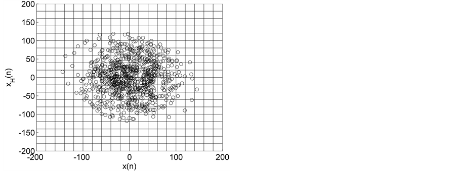 (b)
(b)
Figure 1. HTSPs with matrix partitions, for EEG signals from normal subjects (a) EO state (set A) and (b) EC state (set B).
Compor FC can serve as a measure of the complexity as well as a measure of dispersion of points in the scatter plot. A larger value of DispComp indicates an increased complexity and degree of variability, while a smaller value indicates decreased complexity and more concentration of points in certain portions of the scatter plot. The variability seen in the HTSP plot gets manifested in the DispComp or FC. A time series where the approximate first order time derivatives are changing smoothly will have a lower DispComp (higher FC), while an irregular time series will have a higher DispComp (lower FC). Changes in frequency content during different EEG states get reflected in the DispComp. The degree of variability in EEGs of different physiopathological states was found by comparing the mean values of DispCompin respective states. Instead of DispComp, we can also use FC to interpret variability in the HTSP. In this case, the more is the FC the lower is the variability and vice versa.
2.5. Statistical Analysis and Receiver Operating Characteristic (ROC) Analysis
Statistical significance for the differences between the different non-seizure and seizure classes was assessed using independent-samples significance tests (Student’s t-tests). A p < 0.0001 was considered significantly different. In case, if significant differences between classes are found, then the ability of the nonlinear analysis method to discriminate non-seizure and seizure states is evaluated using receiver operating characteristic (ROC) plots in terms of area under ROC (AUC) and the following performance parameters: sensitivity, specificity, precision, and accuracy. ROC plots are used to gauge the predictive ability of a classifier over a wide range of values [35] . A threshold value is applied such that a feature value below this threshold will be assigned one category while a feature value above the threshold will be assigned other category. ROC curves are obtained by plotting sensitivity values (which represent that proportion of states identified as seizure) along the y axis against the corresponding (1-specificity) values (which represent the proportion of the correctly identified non- seizure states) for all the available cutoff points along the x axis. Accuracy is a related parameter that quantifies the total number of states (both non-seizure and seizure states) precisely classified. The AUC measuresthis discrimination, that is, the ability of the test to correctly classify non-seizure and seizure classes and is regarded as an index of diagnostic accuracy. The optimum threshold is the cut-off point in which the highest accuracy (minimal false negative and false positive results) is obtained. This can be determined from the ROC curve as the closet value to the left top point (corresponding to 100% sensitivity and 100% specificity). An AUC value of 0.5 indicates that the test results are better than those obtained by chance, where as a value of 1.0 indicates a perfectly sensitive and specific test. A rough guide to classify the precision of a diagnostic test based on AUC is as follows: If the AUC is between 0.9 and 1.0, then the results are treated to be excellent; If the AUC is between 0.8 and 0.89, then the results are treated to be good; the results are fair for values between 0.7 and 0.79; the results are poor for values between 0.6 and 0.69; If the AUC is between 0.5 and 0.59, then the outcome is treated to be bad.
2.6. Surrogate Data Testing
If the dynamics that generated the time series is not known or if the time series is noisy, in that case it is essential to investigate whether the amount of nonlinear deterministic dependencies is worth analyzing further or to treat the time series as stochastic. Hence, one of the first steps before applying the nonlinear technique to the data is to investigate if the application of such technique is justified and useful. If an experimental time series of limited length and finite precision is given, which is true in practice, it may be impossible to distinguish between nonlinear and linear dynamics due to stochastic components. The main reason behind this rationale is that linear stochastic processes can generate very complicated looking signals and that not all the structures that we observe in the data are likely to be due to nonlinear dynamics of the system. The method of surrogate data testing, introduced by Theiler et al. [36] , has been a popular validating test to address this issue. This test facilitates to find out if the irregularity of the data is most likely due to nonlinear deterministic structure or due to variations in system parameters or due to random inputs to the system.
This section presents a brief sketch of the idea in that connection. The starting point is to create an ensemble of random nondeterministic surrogate data sets that have the same mean, variance, and power spectrum as the original time series, but has no further determinism built in. The measured topological properties of the surrogate data sets are compared with those of the original time series. If, in case, the surrogate data sets and original data yield the same values for the topological properties (within the standard deviation of the surrogate data sets) then the null hypothesis that the original data is random noise cannot be ruled out. On the other hand, if the data under test is generated by a nonlinear process, the value for the topological property would be different from that of the surrogate data, and the null hypothesis that a linear method characterizes the data can be rejected.
Surrogate data completely destroy the sequential order of the original time series, while preserving the first and second order moments of the original series [36] . The method of computing surrogate data sets with the same mean, variance, and power spectrum as the original time series, but otherwise random is as follows: First find the Fourier transform of the original time series, then randomize the phases, and find the inverse Fourier transform. The resulting time series is that of the surrogate data. More details can be found in [36] . However, Rapp et al. have shown that inappropriately constructed random phase surrogates can lead to false-positive rejections of the surrogate null hypothesis [37] . They found that numerical errors in the computation of Fourier transform was the cause for this problem and that Welch windowing the data can eliminate false-positive rejections of the surrogate null hypothesis. Hence, in this study, we made sure that Welch window was introduced before the computation of the Fourier transform of the EEG segment whose surrogate needs to be found.
3. Results and Discussion
First, we evaluated the ability of the DispEntropy, DispComp, and FC, in discriminating EEGs from Bonn Database, into non-seizure (normal or nonictal) and seizure (ictal) classes. This encompasses the important discriminations in the medical field related to epilepsy, such as seizure warning systems or closed-loop seizure control systems [38] . We averaged the respective values of DispEntropy, DispComp, and FC, for the five individual EEG states from the five sets in the Bonn database and the distribution of DispEntropy, DispComp, and FC values were plotted in a box and whisker diagram. Independent-samples t-tests were used to evaluate statistical differences between different non-seizure and seizure classes. If significant differences between classes were found, then the ROC analysis was performed to assess the diagnostic ability of these nonlinear methods.
When analyzing an EEG signal, it is customary to segment a long signal into short windows of length W and compute the measure of interest for each window. A thumb rule to select window length is that W must be long enough to reliably estimate the measure of interest (for example, DispEntropy, in this context), while W must be short enough to accurately capture local activities, like seizures. In this study, the EEG signal is segmented using a moving window analysis technique. The length of each segment is about 5 sec (870 samples) with no overlap between adjacent windows along the whole EEG recording.
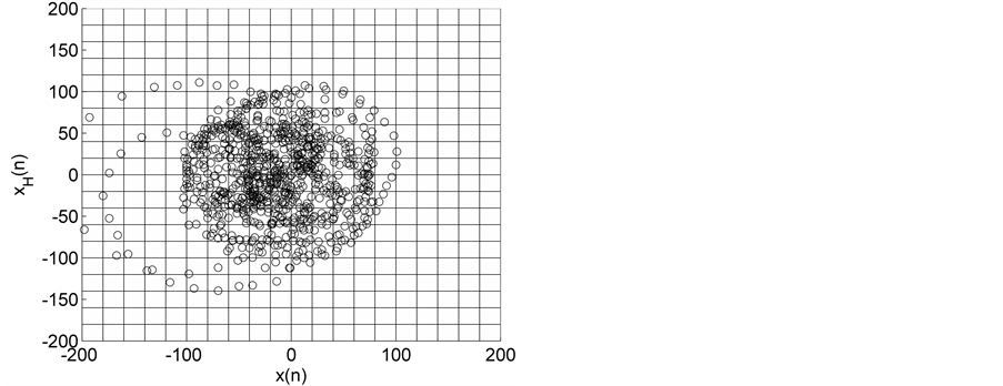
Representative HTSPs for the different EEG states, one from each of the five sets, are shown in Figure 1 and Figure 2. Figure 1(a) and Figure 1(b) show, respectively, HTSPs for EO and EC EEG signals from normal subjects (sets A and B). The plots clearly show differences between the two states. The points corresponding to EO state tend to be located close around the origin, while those corresponding to EC state are comparatively spread in the diagram. This implies that the EEG variability in brain activity is increased when the eyes are closed compared to that when eyes are open in the same subject. This can be attributed to changes in frequency content and degrees of freedom in the corresponding EEG signals as the mental state is switched from one to another. Figures 2(a)-(c) show, respectively, HTSPs for inter-ictal states (from hippocampal formation of the opposite hemisphere of the brain), inter-ictal states (within epileptogenic zone), and ictal states (sites exhibiting seizure activity) of epileptic subjects (sets C, D, and E). The plots clearly show differences between the two states, non-seizure and seizure. The points corresponding to inter-ictal state, in Figure 2(a) and Figure 2(b), tend to be located close around the origin, while those corresponding to ictal state, in Figure 2(c), are widely spread in the diagram. This implies that the EEG variability in brain activity is increased drastically when in the ictal state compared to that when in the inter-ictal state. This can be attributed to changes in frequency content and degrees of freedom in the corresponding EEG signals as the mental state is switched from chaos to order. Comparing HTSPs in Figure 1(a), Figure 1(b), Figures 2(a)-(c) the following conclusions can be drawn: 1) Least degree of variability is found in the inter-ictal states, while highest degree of variability can be found in ictal states. 2) The degree of variability in normal EEG states is higher than that of inter-ictal states, while considerably lower than that of ictal state. Now we quantify these conclusions for the entire Bonn database using DispEntropy, DispComp, and FC. Figures 3(a)-(c) depict respectively, the distribution of DispEntropy, DispComp, and FC values for the five individual EEG states belonging to the different sets in the Bonn database through the box and whisker plots. The results of statistical analysis of independent-samples t-tests for each pair of non-seizure and seizure classes are shown in the second column of Tables 1-3. Since very significant statistical differences between classes were found (p < 0.0001), the ROC analyses were performed to assess the diagnostic ability of this nonlinear method. The descriptive results for AUC, average sensitivity, average specificity, average precision, and average accuracy are summarized in the columns three through seven of the same Tables 1-3. From the tables it is very clear that all three measures, DispEntropy, DispComp, and FC, can readily discriminate between seizure and non-seizure states with very high accuracy.
Before proceeding further, we assess the appropriateness of applying the above nonlinear techniques through surrogate data analysis. We generated an ensemble of 20 surrogates for each EEG signal, as mentioned in Section 2.5. DispEntropy, DispComp, and FC were computed for each surrogate and averaged to obtain the corresponding mean Disp Entropy, mean DispComp, and mean FC of the respective surrogate data set. We compared the DispEntropy, DispComp, and FC results from the original data with the corresponding mean DispEntropy, DispComp, and FC results from the ensemble surrogate data using paired t-tests. The statistical results are shown in Tables 4-6, which reveal significant differences between original data and their surrogate in each dataset. This implies that variation inherent in the EEG data was not due to random fluctuations, but instead is more likely due to the consequences of some deterministic process. These findings confirm the appropriateness of applying the above DispEntropy, DispComp, and FC nonlinear analysis to the EEG data.
In this study, to explore the robustness of DispEntropy and DispComp further, in discriminating non-seizure and seizure we went one step ahead to apply this nonlinear method on EEG data from CHB-MIT scalp EEG database and compare the evolution of these quantifiers with time, and evaluate the performance with those of two popularly employed features in epilepsy detection: sample entropy (SampEn) and approximate entropy (ApEn). Details about ApEn and SampEn are beyond the scope of this paper and can be found in Ref [39] - [42] . Since DispComp and FC are related, evolution of FC is not discussed in this section. Figure 4 compares the performance and evolution of Disp Entropy and Disp Comp with that of SampEn, for a patient labeled chb01_26_edf
 (a)
(a)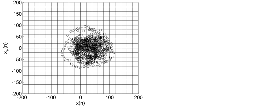 (b)
(b)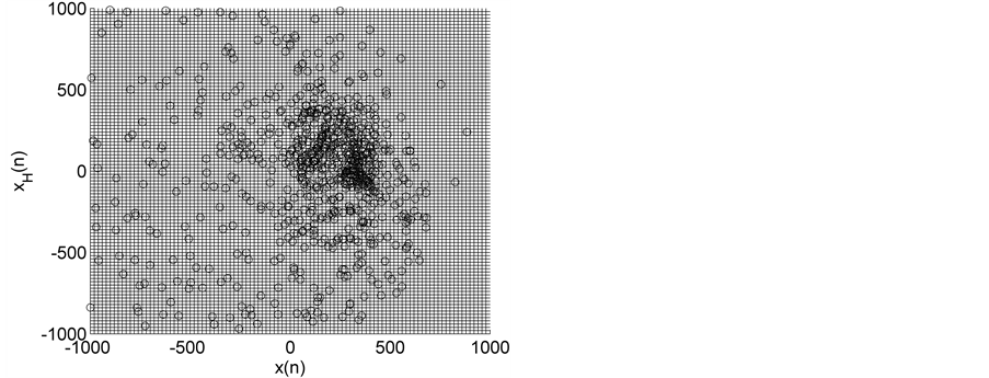 (c)
(c)
Figure 2. HTSPs with matrix partitions, for EEG signals from epileptic subjects (a) inter-ictal state S (set C), (b) inter-ictal state S1 (set D), and (c) ictal state SZ (set E).
randomly selected from CHB-MIT scalp EEG database. Figure 4(a) shows the seizure evolution profile of chb01_26_edf around the occurrence of the seizure. The vertical lines mark the start and end timings of the occurrence of a seizure determined by medical experts. An epileptic seizure time series has transients at the begin-
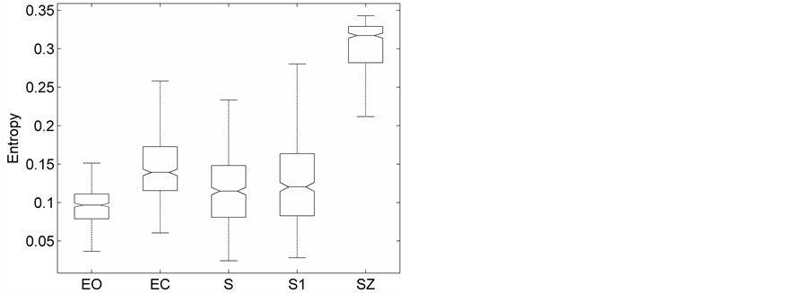 (a)
(a)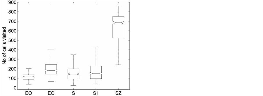 (b)
(b)
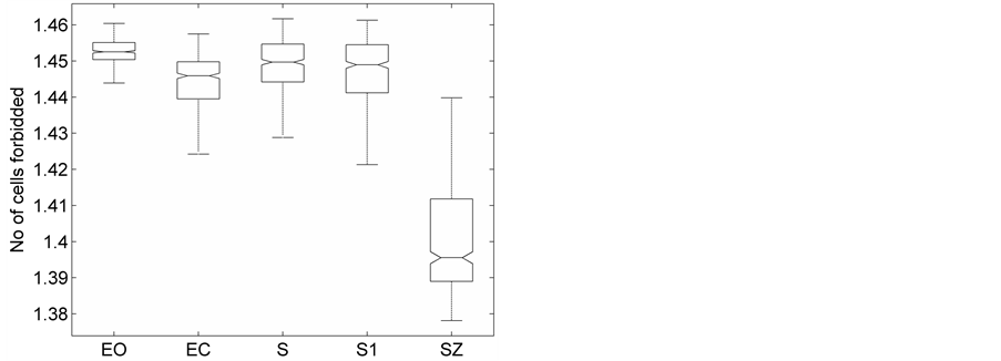 (c)
(c)
Figure 3. The distribution of the (a) DispEntropy, (b) DispComp, and (c) FC corresponding to five sets of EEG states using Box-whiskers plots (without outliers).
ning and at the end. The seizure becomes more regular and coherent in the middle part. Let us examine the variation of Disp Entropy and Disp Comp with time as seizure progresses. At the onset of seizure, as seen from Figure 4(b) and Figure 4(c), DispEntropy and DispComp increase gradually to higher values and remain almost constant during mid-seizure. After the seizure offset, both decrease gradually to the lower inter-ictal background

Table 1. Descriptive results of independent-samples t-tests and ROC analysis on DispEntropy for discriminating different non-seizure and seizure classes.
Table 2. Descriptive results of independent-samples t-tests and ROC analysis on DispComp for discriminating different non-seizure and seizure classes.
Table 3. Descriptive results of independent-samples t-tests and ROC analysis on FC for discriminating different non-seizure and seizure classes. Since DispComp and FC exhibit a kind of inverse relationship statistical comparison in Table 2 and Ta- ble 3 yields the similar results.
Table 4. Distribution of DispEntropy of Bonn EEG data (All values are expressed as mean ± SD); Descriptive results of paired-samples t-tests on DispEntropy for discriminating EEG datasets and their surrogates.
value. This implies that during seizure the complexity and degree of variability associated with EEG increases to a higher level from that of the background value. Slightly after seizure offset, complexity as well as variability return to the background level. Obviously, when away from the seizure the EEG shows lower complexity and less degree of variability. The dynamic range of DispComp being large, it becomes easy to separate properly non-seizure and seizure states.
Unlike DispEntropy and DispComp, at the onset of seizure, as seen from Figure 4(d), the sample entropy SampEn, drops slightly first on seizure onset, followed by an increase, then an almost constant level during mid- seizure. This is followed by a decrease to the background value by the end of the seizure. This is attributed to the
Table 5. Distribution of DispComp of Bonn EEG data (All values are expressed as mean ± SD); Descriptive results of paired-samples t-tests on DispComp for discriminating EEG datasets and their surrogates.
Table 6. Distribution of FC of Bonn EEG data (All values are expressed as mean ± SD); Descriptive results of paired-sam- ples t-tests on FC for discriminating EEG datasets and their surrogates.
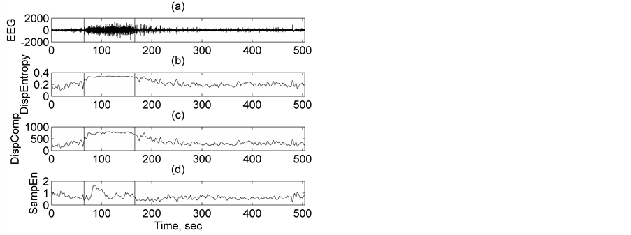
Figure 4. Comparison of the performance and evolution (with time) of DispEntropy, DispComp, and FC, with that of SampEn, for a patient labeled chb01_26_edf.
fact that entropy is a measure of irregularity of the time series and during epilepsy the irregularity of EEG increases and then decreases considerably [20] [39] [40] . The dynamic range being small in the case of Disp Entropy or SampEn, it becomes difficult to discriminate properly non-seizure and seizure states. Electrographic changes are visible in all the three features in Figure 4. But among the three quantifiers, DispComp shows a better manifestation of the onset and offset of seizure epoch. As a second representative demonstration, Figure 5 compares the performance and evolution of DispEntropy and DispComp with that of ApEn, for a patient labeled chb05_16_edf randomly chosen from CHB-MIT scalp EEG database. The interpretation for the different plots in Figure 4 can very well be extended to respective plots in Figure 5 (with SampEn replaced by ApEn) and similar conclusions can be drawn, as the behavior of the features is identical in either case. Again, it is found that among the three quantifiers, DispComp shows a better manifestation of the onset and offset of seizure epoch. Further, it is to be emphasized that DispComp has the advantage of easy implementation and fast computation. All these considerations show that this nonlinear method is a suitable approach for automatic seizure detection. Although
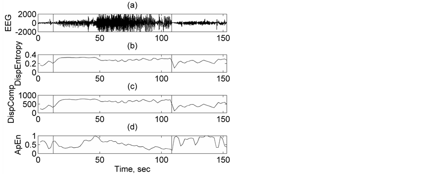
Figure 5. Comparison of the performance and evolution (with time) of DispEntropy, DispComp, and FC, with that of ApEn, for a patient labeled chb05_16_edf.
these results suggest that DispEntropy and DispComp (or FC) can detect epileptic seizures from scalp EEG recordings too, further work must be carried out to prove the possible usefulness of this technique in seizure prediction.
The principal findings of this study are: 1) DispEntropy/DispComp is increased when eyes are closed in normal subjects compared to that when eyes are open. This means variability in EEG is enhanced when eyes are closed compared to that when eyes are open. 2) DispEntropy/DispComp, in epileptic patients, during ictal state is considerably increased compared to that in inter-ictal state. This implies that variability in EEG significantly increases during ictal state. 3) DispEntropy/DispComp can readily discriminate among different physiological and pathological states in intracranial as well as scalp EEGs. 4) A comparison of time evolution among DispEntropy/DispComp, ApEn, and SampEn, shows that DispEntropy/DispComp outperforms others in the detection of onset and offset of seizures. 5) The suitability of employing the above nonlinear technique is justified through surrogate data analysis. We think that DispEntropy/DispCompis most promising in providing new insight into the evolution of chaos or variability of underlying brain activity. Of course, between DispComp and DispEntropy, DispComp overrides DispEntropy because the former has the advantage of easy implementation and fast computation.
4. Conclusion
There is strong evidence that the mechanisms generating EEG obey nonlinear deterministic laws and that these processes are chaotic. This study on chaotic analysis of EEG time series from healthy and epileptic subjects using newly defined DispEntropy, DispComp, and FC, show promise not only in the discrimination of different physiological and pathological brain states, but also in providing new insight into the evolution of chaos or variability of underlying brain activity. The appropriateness of applying the above nonlinear technique is justified through surrogate data analysis. Of course, future work must be carried out to prove the possible usefulness of this technique in seizure prediction.
Conflict of Interests
The author(s) declare(s) that there is noconflict of interests regarding the publication of this article.
Cite this paper
Chandrakar Kamath, (2015) Analysis of EEG Dynamics in Epileptic Patients and Healthy Subjects Using Hilbert Transform Scatter Plots. Open Access Library Journal,02,1-14. doi: 10.4236/oalib.1100745
References
- 1. Bethesda, M.D. (2004) Seizures and Epilepsy: Hope through Research. National Institute of Neurological Disorders and Stroke (NINDS), 2004.
http://www.ninds.nih.gov Goy/health and medical/pubs/seizures and epilepsy htr.htm, NINDS. - 2. Logar, C., Walzl, B. and Lechner, H. (1994) Role of Long-Term EEG Monitoring in Diagnosis and Treatment of Epilepsy. European Neurology, 34, 29-32.
http://dx.doi.org/10.1159/000119506 - 3. Adeli, H., Ghosh-Dastidar, S. and Dadmehr, N. (2007) A Wavelet-Chaos Methodology for Analysis of EEGs and EEG Sub-Bands to Detect Seizure and Epilepsy. IEEE Transactions on Biomedical Engineering, 54, 205-211.
http://dx.doi.org/10.1109/TBME.2006.886855 - 4. Iasemidis, L.D., Sackellares, J.C., Zaveri, H.P. and Williams, W.J. (1990) Phase Space Topography and the Lyapunov Exponent of the Electrocorticogram in Partial Seizures. Brain Topography, 2, 187-201.
http://dx.doi.org/10.1007/BF01140588 - 5. Iasemidis, L.D. and Sackellares, J.C. (1990) Long Time Scale Spatio-Temporal Patterns of Entrainment in Preictalecog Data in Human Temporal Lobe Epilepsy. Epilepsia, 31, 621.
- 6. Iasemidis, L.D. (1991) On the Dynamics of the Human Brain in Temporal Lobe Epilepsy. Ph.D. Dissertation, University of Michigan.
- 7. Iasemidis, L.D. and Sackellares, J.C. (1991) The Evolution with Time of the Spatial Distribution of the Largest Lyapunov Exponent on the Human Epileptic Cortex. In: Duke, D. and Pritchard, W., Eds., Measuring Chaos in the Human Brain, World Scientific, Singapore, 49-82.
- 8. Iasemidis, L.D. and Sackellares, J.C. (1996) Chaos Theory and Epilepsy. The Neuroscientist, 2, 118-126.
http://dx.doi.org/10.1177/107385849600200213 - 9. Iasemidis, L.D., Principe, J.C. and Sackellares, J.C. Measurement and Quantification of Spatiotemporal Dynamics of Human Epileptogenic Seizures. In: Akay, M., Ed., Nonlinear Biomedicalsignal Processing, IEEE Press, in Press.
- 10. Sackellares, J.C., Iasemidis, L.D., Shiau, D.S., Gilmore, R.L. and Roper, S.N. (2000) Epilepsy—When Chaos Fails. In: Lehnertz, K., Arnhold, J., Grassberger, P. and Elger, C.E., Eds., Chaos in Brain? World Scientific, Singapore, 112-133.
- 11. Klonowski, W., Jernajczyk, W., Niedzielska, K., Rydz, A. and Stepien, R. (1999) Quantitative Measure of Complexity of EEG Signal Dynamics. Acta Neurobiologiae Experimentalis, 59, 315-321.
- 12. Theiler, J. and Rapp, P.E. (1996) Re-Examination of the Evidence for Low-Dimensional, Nonlinear Structure in the Human Electroencephalogram. Electroencephalography and Clinical Neurophysiology, 98, 213-222.
- 13. Jeong, J. (2004) EEG Dynamics in Patients with Alzheimer’s Disease. Clinical Neurophysiology, 115, 1490-1505.
http://dx.doi.org/10.1016/j.clinph.2004.01.001 - 14. Shaw, R. (1981) Strange Attractors, Chaotic Behavior, and Information Flow. Zeitschrift für Naturforschung A, 36, 80-112.
- 15. Li, X.L., Ouyang, G.X. and Richards, D.A. (2007) Predictability Analysis of Absence Seizures with Permutation Entropy. Epilepsy Research, 77, 70-74.
http://dx.doi.org/10.1016/j.eplepsyres.2007.08.002 - 16. Pravin Kumar, S., Sriraam, N. and Benakop, P.G. (2008) Automated Detection of Epileptic Seizures Using Wavelet Entropy Feature with Recurrent Neural Network Classifier. Proceedings of the 2008 IEEE Region 10 Conference of TeNCON, Hyderabad, 19-21 November 2008, 1-5.
- 17. Ocak, H. (2009) Automatic Detection of Epileptic Seizures in EEG Using Discrete Wavelet Transform and Approximate Entropy. Expert Systems with Applications, 36, 2027-2036.
http://dx.doi.org/10.1016/j.eswa.2007.12.065 - 18. Ghosh-Dastidar, S., Adeli, H. and Dadmehr, N. (2007) Mixed-Band Wavelet-Chaos-Neural Network Methodology for Epilepsy and Epileptic Seizure Detection. IEEE Transactions on Biomedical Engineering, 54, 1545-1551.
http://dx.doi.org/10.1109/TBME.2007.891945 - 19. Alam, S.M.S., Bhuiyan, M.I.H., Aurangozeb and Shahriar, S.T. (2012) EEG Signal Discrimination Using Non-Linear Dynamics in the EMD Domain. International Journal of Computer and Electrical Engineering, 4, 326-330.
http://dx.doi.org/10.7763/IJCEE.2012.V4.505 - 20. Radhakrishnan, N. and Gangadhar, B.N. (1998) Estimating Regularity in Epileptic Seizure Time Series Data—A Complexity Measure Approach. IEEE Engineering in Medicine and Biology Magazine, 17, 89-94.
http://dx.doi.org/10.1109/51.677174 - 21. Hu, J., Gao, J. and Principe, J. (2006) Analysis of Biomedical Signals by the Lempel-Ziv Complexity: The Effect of Finite Data Size. IEEE Transactions on Biomedical Engineering, 53, 2606-2609.
http://dx.doi.org/10.1109/TBME.2006.883825 - 22. Gao, J., Hu, J. and Tung, W. (2011) Complexity Measures of Brain Wave Dynamics. Cognitive Neurodynamics, 5, 171-182.
- 23. Doyle, T.L.A., Dugan, E.L., Brendan Humphries, B. and Newton, R.U. (2004) Discriminating between Elderly and Young Using a Fractal Dimension Analysis of Centre of Pressure. International Journal of Medical Sciences, 1, 11-20.
http://dx.doi.org/10.7150/ijms.1.11 - 24. Eckmann, J.P. and Ruelle, D. (1992) Fundamental Limitations for Estimating Dimensions and Lyapunov Exponents in Dynamical Systems. Physica D, 56, 185-187.
http://dx.doi.org/10.1016/0167-2789(92)90023-G - 25. Klonowski, W., Stepien, R., Olejarczyk, E., Jernajczyk, W., Niedzielska, K. and Karlinski, A. (1999) Chaotic Quan tifiers of EEG-Signal for Assessing Photo and Chemo-Therapy. Medical & Biological Engineering & Computing, 37, 436-437.
- 26. Andrzejak, R.G., Lehnertz, K., Rieke, C., Mormann, F., David, P. and Elger, C.E. (2001) Indications of Nonlinear Deterministic and Finite Dimensional Structures in Time Series of Brain Electrical Activity: Dependence on Recording Region and Brain State. Physical Review E, 64, Article ID: 061907.
http://dx.doi.org/10.1103/PhysRevE.64.061907 - 27. CHB-MIT Scalp EEG Database [Online].
http://physionet.org/physiobank/database/chbmit/ - 28. Le Van Quyen, M., Foucher, J., Lachaux, J., Rodriguez, E., Lutz, A., Martinerie, J. and Varela, F. (2001) Comparison of Hilbert Transform and Wavelet Methods for the Analysis of Neuronal Synchrony. Journal of Neuroscience Methods, 111, 83-98.
http://dx.doi.org/10.1016/S0165-0270(01)00372-7 - 29. Quiroga, R.Q., Kraskov, A., Kreuz, T. and Grassberger, P. (2002) Performance of Different Synchronization Measures in Real Data: A Case Study on Electroencephalographic Signals. Physical Review E, 65, 1-15.
- 30. Kamen, P.W. and Tonkin, A.M. (1995) Application of the Poincaré Plot to Heart-Rate-Variability—A New Measure of Functional Status in Heart Failure. Australian and New Zealand Journal of Medicine, 25, 18-26.
http://dx.doi.org/10.1111/j.1445-5994.1995.tb00573.x - 31. Cohen, M.E., Hudson, D.L. and Deedwania, P.C. (1996) Applying Continuous Chaotic Modeling to Cardiac Signal Analysis. IEEE Engineering in Medicine and Biology Magazine, 15, 97-102.
http://dx.doi.org/10.1109/51.537065 - 32. Hornero, R., Abásolo, D., Jimeno, N., Sánchez, C.I., Poza, J. and Aboy, M. (2006) Variability, Regularity, and Complexity of Time Series Generated by Schizophrenic Patients and Control Subjects. IEEE Transactions on Biomedical Engineering, 53, 210-218.
http://dx.doi.org/10.1109/TBME.2005.862547 - 33. Cohen, M.E. and Hudson, D.L. (2001) Inclusion of ECG and EEG Analysis in Neural Network Models. Proceedings of the 23rd International Conference of the IEEE Engineering in Medicine and Biology Society (EMBC), 2, 1621-1624.
- 34. Thuraisingham, R.A., Tran, Y., Boord, P. and Craig, A. (2007) Analysis of Eyes Open, Eye Closed EEG Signals Using Second-Order Difference Plot. Medical & Biological Engineering & Computing, 45, 1243-1249.
http://dx.doi.org/10.1007/s11517-007-0268-9 - 35. Zweig, M.H. and Campbell, G. (1993) Receiver-Operating Characteristic (ROC) Plots: A Fundamental Evaluation Tool in Clinical Medicine. Clinical Chemistry, 39, 561-577.
- 36. Theiler, J., Eubank, S., Longtin, A., Galdrikian, B. and Farmer, J.D. (1992) Testing for Nonlinearity in Time Series: The Method of Surrogate Data. Physica D, 58, 77-94.
http://dx.doi.org/10.1016/0167-2789(92)90102-S - 37. Rapp, P.E., Cellucci, C.J., Watanabe, T.A.A., Albano, A.M. and Schmah, T.I. (2001) Surrogate Data Pathologies and the False-Positive Rejection of the Null Hypothesis. International Journal of Bifurcation and Chaos, 11, 983-997.
http://dx.doi.org/10.1142/S021812740100250X - 38. Stacey, W.C. and Litt, B. (2008) Technology Insight: Neuroengineering and Epilepsy-Designing Devices for Seizure Control. Nature Clinical Practice Neurology, 4, 190-201.
- 39. Richmann, J.S. and Moorman, J.R. (2000) Physiological Time-Series Analysis Using Approximate Entropy and Sample Entropy. American Journal of Physiology. Heart and Circulatory Physiology, 278, H2039-H2049.
- 40. Lake, D.E., Richman, J.S., Griffin, M.P. and Moorman, J.R. (2002) Sample Entropy Analysis of Neonatal Heart Rate Variability. American Journal of Physiology. Regulatory, Integrative and Comparative Physiology, 283, R789-R797.
- 41. Ramdani, S., Seigle, B., Lagarde, J., Bouchara, F. and Bernard, P.L. (2009) On the Use of Sample Entropy to Analyze Human Postural Sway Data. Medical Engineering & Physics, 31, 1023-1031.
http://dx.doi.org/10.1016/j.medengphy.2009.06.004 - 42. Song, Y. and Liò, P. (2010) A New Approach for Epileptic Seizure Detection: Sample Entropy Based Feature Extraction and Extreme Learning Machine. Journal of Biomedical Science and Engineering, 3, 556-567.
http://dx.doi.org/10.4236/jbise.2010.36078 - 43. Liang, S., Wang, H. and Chang, W. (2010) Combination of EEG Complexity and Spectral Analysis for Epilepsy Diagnosis and Seizure Detection. EURASIP Journal on Advances in Signal Processing, 2010, 1-15.