Creative Education
2011. Vol.2, No.3, 292-295
Copyright © 2011 SciRes. DOI:10.4236/ce.2011.23040
Teaching PCA through Letter Recognition
Tanja Van Hecke
Faculty of Applied Engineering Sciences, University College Ghent, Ghent, Belgium.
Received February 8th, 2011; revised March 14th, 2011; accepted April 2nd, 2011.
This article presents the use of a real life problem to reach a deeper understanding among students of the benefits
of principal components analysis. Pattern recognition applied on the 26 letters of the alphabet is a recognizable
topic for the students. Moreover it is still verifiable with computer algebra software. By means of well defined
exercises the student can be guided in an active way through the learning process.
Keywords: Data Reduction, Eigenvalues, Eigenvectors
Introduction
Principal Components Analysis (PCA) is a statistical tech-
nique for data reduction which is taught to students mostly with
a pure mathematical approach. This paper describes how teach-
ers can introduce students to the concepts of principal compo-
nents analysis by means of letter recognition. The described
approach is one of an active learning environment (with
hands-on exercises can be implemented in the classroom), a
platform to engage students in the learning process and may
increase student/student and student/instructor interaction. The
activities require use of some basic matrix algebra and eigen-
value/eigenvector theory. As such they build on knowledge
students have acquired in matrix algebra classes.
Former attempts to develop a more creative instruction ap-
proach for PCA can be found with Dassonville and Hahn
(Dassonville, 2000). They developed a CD-rom geared to the
teaching of PCA for business school students. The test of this
pedagogical tool showed that this new approach, based on dy-
namic graphical representations, eased the introduction to the
field, yet did not foster more effective appropriation of those
concepts. Besides, when the program was used in self tuition
mode, the students felt disconnected from the class environ-
ment, as Dassonville and Hahn claim themselves.
A second initiative is DoLStat@d (Mori, 2003), developed at
Okayama University in Japan by Yuichi Mori and colleagues.
This web based learning system, available online at
http://mo161.soci.ous.ac.jp/@d/DoLStat/index.html, provides
real world data with their analysis stories about various topics,
PCA included. Since only applications are presented, without
any background information about the method itself, students
unfamiliar to PCA, will not reach a deeper understanding about
PCA and will keep stabbing at a recipe approach.
Principal Components Analysis
The objective of PCA (Jackson, 2003) is to obtain a
low-dimensional representation of the objects/individuals with
minimum information loss, which facilitates compression of the
initial data and extracting the most relevant characteristics.
PCA is a known data reduction technique in statistical pat-
tern recognition and signal processing (Kastleman, 1996) (Turk,
1991). It is valuable because it is a simple non-parametric
method of extracting relevant information from confusing
datasets. PCA is also called the Karhunen-Loeve Transform
(KLT, named after Kari Karhunen (Karhunen, 1947) & Michel
Loève (Loève, 1978)) or the Hotelling Transform (Hotelling,
1935).
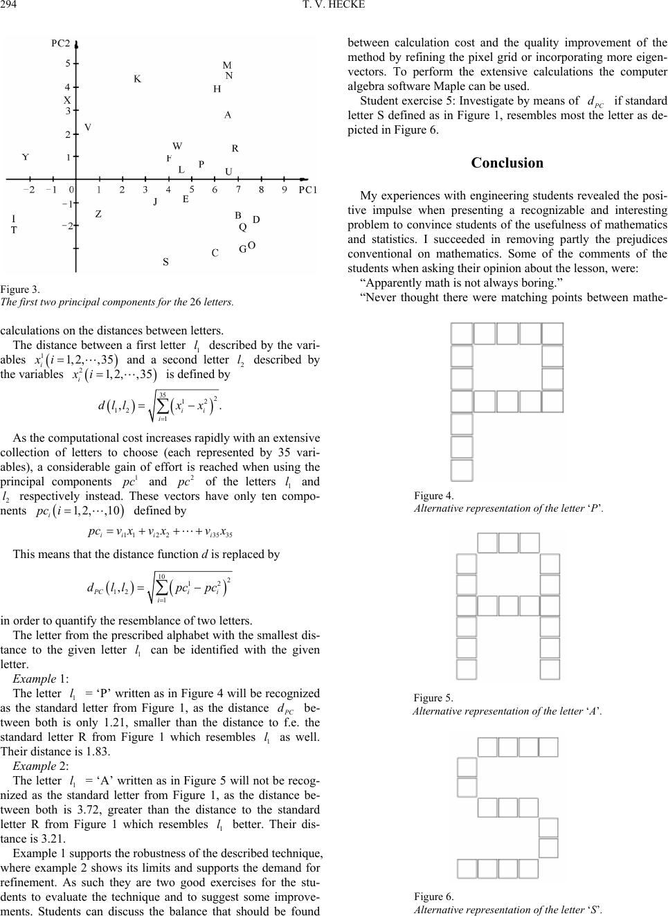
PCA involves finding eigenvalues and corresponding eigen-
vectors of the data set, using the covariance matrix. The corre-
sponding eigenvalues of the matrix give an indication of the
amount of information the respective principal components
represent. The methodology for calculating principal compo-
nents is given by the following algorithm.
Let 12
,,,
m
x
xx be the variables.
 Computation of the global means i
x


1, 2,,im
 Computation of the sample covariance matrix Σ of di-
mension mm

 Computation of the eigenvalues and eigenvectors of Σ
 Keep only the n eigenvectors


12
,,,
ii im
vv v
i
v


1, 2,,in corresponding to the largest eigenvalues. Then


11 21, 2,, ii n are called principal com-
ponents.
2
vx vx im x
m
v i
Corresponding eigenvectors are uncorrelated and have the
greater variance. In order to avoid the components that have an
undue influence on the analysis, the components are usually
coded with mean as zero and variance as one. This standardiza-
tion of the measurement ensures that they all have equal weight
in the analysis.
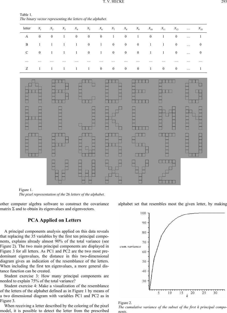
Representation of Letters by Binary Variables
We use the pixel representation with seven rows and five
columns as in Figure 1 for the alphabet. This image is trans-
formed into a binary vector representation (see Table 1). This
was accomplished by using 35 variables i
x
by running the figure from top to down and from left to right
assigning 1 to an occupied pixel and 0 to a non-occupied pixel.

1, 2,, 35i
Student exercise 1: Make the binary vector representation of
the 26 letters of the alphabet (less time consuming: each student
makes one).
Student exercise 2: Use Maple (www.maplesoft.com) or some

T. V. HECKE 293
Table 1.
The binary vector representing the letters of the alphab et.
letter 1
x
2
x
3
x
4
x
5
x
6
x
7
x
8
x
9
x
10
x
11
x
12
x
… 35
x
A 0 0 1 0 0 0 1 0 1 0 1 0 … 1
B 1 1 1 1 0 1 0 0 0 1 1 0 … 0
C 0 1 1 1 0 1 0 0 0 1 1 0 … 0
… … … … … … … … … … … … … … …
Z 1 1 1 1 1 0 0 0 0 1 0 0 … 1
Figure 1.
The pixel representation of the 26 letters of the alphabet.
other computer algebra software to construct the covariance
matrix Σ and to obtain its eigenvalues and eigenvectors.
PCA Applied on Letters
A principal components analysis applied on this data reveals
that replacing the 35 variables by the first ten principal compo-
nents, explains already almost 90% of the total variance (see
Figure 2). The two main principal components are displayed in
Figure 3 for all letters. As PC1 and PC2 are the two most pre-
dominant eigenvalues, the distance in this two-dimensional
diagram gives an indication of the resemblance of the letters.
When including the first ten eigenvalues, a more general dis-
tance function can be created.
Student exercise 3: How many principal components are
needed to explain 75% of the total variance?
Student exercise 4: Make a visualization of the resemblance
of the letters of the alphabet defined as in Figure 1 by means of
a two dimensional diagram with variables PC1 and PC2 as in
Figure 3.
When receiving a letter described by the coloring of the pixel
model, it is possible to detect the letter from the prescribed
alphabet set that resembles most the given letter, by making
Figure 2.
The cumulative variance of the subset of the first k principal compo-
nents.

T. V. HECKE 294
Figure 3.
The first two principal components for the 26 letters.
calculations on the distances between letters.
The distance between a first letter 1 described by the vari-
ables
l


11,2,, 35
i
xi

and a second letter described by
the variables 2
l

21, 2,
i
xi, 35 is defined by
 
35 2
12
12
1
,.
ii
i
dllx x



As the computational cost increases rapidly with an extensive
collection of letters to choose (each represented by 35 vari-
ables), a considerable gain of effort is reached when using the
principal components 1
p
c and 2
p
c of the letters 1 and
2 respectively instead. These vectors have only ten compo-
nents defined by
l
l

1, 2,,1
i
pci 

0
112 235 35ii ii
p
cvxv vxx
This means that the distance function d is replaced by
 
10 2
12
12
1
,
PCi i
i
dll pcpc



in order to quantify the resemblance of two letters.
The letter from the prescribed alphabet with the smallest dis-
tance to the given letter can be identified with the given
letter. 1
l
Example 1:
The letter 1 = ‘P’ written as in Figure 4 will be recognized
as the standard letter from Figure 1, as the distance PC be-
tween both is only 1.21, smaller than the distance to f.e. the
standard letter R from Figure 1 which resembles as well.
Their distance is 1.83.
ld
1
l
Example 2:
The letter 1 = ‘A’ written as in Figure 5 will not be recog-
nized as the standard letter from Figure 1, as the distance be-
tween both is 3.72, greater than the distance to the standard
letter R from Figure 1 which resembles better. Their dis-
tance is 3.21.
l
1
l
Example 1 supports the robustness of the described technique,
where example 2 shows its limits and supports the demand for
refinement. As such they are two good exercises for the stu-
dents to evaluate the technique and to suggest some improve-
ments. Students can discuss the balance that should be found
between calculation cost and the quality improvement of the
method by refining the pixel grid or incorporating more eigen-
vectors. To perform the extensive calculations the computer
algebra software Maple can be used.
Student exercise 5: Investigate by means of PC if standard
letter S defined as in Figure 1, resembles most the letter as de-
picted in Figure 6.
d
Conclusion
My experiences with engineering students revealed the posi-
tive impulse when presenting a recognizable and interesting
problem to convince students of the usefulness of mathematics
and statistics. I succeeded in removing partly the prejudices
conventional on mathematics. Some of the comments of the
students when asking their opinion about the lesson, were:
“Apparently math is not always boring.”
“Never thought there were matching points between mathe-
Figure 4.
Alternative representation of the l etter ‘P’.
Figure 5.
Alternative representation of the l etter ‘A’.
Figure 6.
Alternative representation of the l etter ‘S’.

T. V. HECKE 295
matics and language.”
“Surprising that we can make computers smart by means of
mathematics, since they are able to recognize letters!”
“Granted, today revealed that statistics is more than calculat-
ing the mean of our exam results.”
The discussions I held in class with my engineering students,
resulted in an impressive improvement in their mathematical
comprehension. Moreover the students became aware of the
relevance of reducing the multidimensional datasets to lower
dimensions for analysis by means of principal components
analysis.
References
Dassonville, P., & Hahn, C. (2000). The multimedia tool: A transitional
medium beween the mathematician’s culture and the professional’s
culture in teaching PCA in a business school. In A. Ahmed, J.
Kraemer, & H. Williams (Eds.), Cultural diversity in mathematics
Education (pp. 125-136). United Kingdom: Horwood
Hotelling, H. (1935). The most predictable criterion. Journal of Educa-
tional Psychology, 26 , 139-142. doi:10.1037/h0058165
Jackson, J. E. (2003). A user’s guide to principal components. New
Jersey: Wiley & Sons, Inc..
Karhunen, K. (1947). Über lineare methoden in der wahrscheinli-
chkeitsrechnung. Annales Academiæ Scientiarum Fennicae Series A1,
Mathematica-Physica, 3 7 , 1-79.
Kastleman, K. (1996). Digital image processing. London: Prentice
Hall.
Loève, M. (1978). Probability theory Vol. II, graduate texts in mathe-
matics 46 (4th ed.). New York, NY: Springer-Verlag.
Mori, Y., Yamamoto, Y., & Yadohisa, H. (2003). Data-oriented learn-
ing system of statistics based on analysis scenario/story (DoLStat).
Bulletin of the International Statistical Institute (ISI), 54th Session
Proceedings, Volume LX Two Books, Book 2 (pp. 74-77).
Turk, M., & Pentland, A. (1991). Eigenfaces for Recognition. Journal
of Cognitive Neurosicence, 3, 71-86. doi:10.1162/jocn.1991.3.1.71