Applied Mathematics, 2011, 2, 1011-1018
doi:10.4236/am.2011.28140 Published Online August 2011 (http://www.SciRP.org/journal/am)
On Generalized Multivalued Random Variational-Like
Inclusions
Mohammad Kalimuddin Ahmad, Salahuddin
Department of Mat hematics, Aligarh Muslim University, Aligarh, India
Received April 9, 2011; revised May 28, 2011; accepted J une 6, 2011
Abstract
In this paper, we posed a random iterative algorithm for generalized multivalued random variational like in-
clusions. We define the random relaxed Lipschitz and relaxed monotone mappings and prove the existence
and convergence of solutions of the random iterative sequences generated by a random iterative algorithm.
Keywords: Generalized Multivalued Random Variational Like Inclusions, Random Iterative Sequences,
Measurable Space, Separable Real Hilbert Space,

-Subdifferential, Hausdorff Metric
1. Introduction
It is well know that the study of random equations in-
volving random operators in view of their need in deal-
ing with probabilistic models in applied sciences is very
important. It has also been well documented that the in-
troduction of the randomness leads to several questions
including the measurability and probabilistic aspect of
solutions [1-4].
The systematic study of random equations employing
the techniques of func tional analysis was first introduced
by Prague school of probabilistic by Spacek [5] and Hans
[6]. This has received considerable attention from nume-
rous authors, e.g. Adomian [7], Tsokos and Padgett [8],
Cho et al. [9], and Chang and Huang [10]. The main
question concerning random operator equations are es-
sen- tially the same as those of deterministic operator
equa- tions, that is question of existence, uniqueness,
characteri- zation, contraction and approximation of so-
lutions. The theory of randomness, however leads to
several new questions like measurability of solutions,
probabilistic and statistical aspects of random solutions,
estimate for the difference between the mean value of the
solutions of the random equations and deterministic so-
lutions of the averaged equations.
The theory of variational inequality provides a natural
and elegant framework for study of many seemingly un-
related free boundary value problems arising in various
branches of engineering, mathematics and financial sci-
ences. Variational inequalities have many deep results
dealing with nonlinear partial differential equations
which play important and fundamental role in general
equilibrium theory, economics, managerial sciences and
operation research, see [11,12].
Motivated and inspired by the recent research work
going in these fields [13-17], we consider the generalized
multivalued random variational like inclusions and con-
struct its random iterative algorithm. Then we prove the
existence and convergence of random solutions of the
problem and establish its equivalence with original pro-
blem.
2. Preliminaries
Let (,)

 be a measurable space and
H
a separable
real Hilbert space whose inner product and norm are
designed by 2 ,=
x
xx . We denote by


B,2
H
H
and


CH , the class of Borel

-field in ,
H
the
family of all nonempty power subsets of
H
and the
family of all nonempty compact subsets of ,
H
respec-
tively.
A mapping :
x
H

 is said to be measurable if for
any


BBH,




,txtB


H
. A mappi ng
:TH

is called random operator if for any
x
H

,




xt,=Ttx
Tis measurable. A random operator is said to be continuous if for any , the mapping t


,:Tt H H
:2
is continuous. A multivalued mapping
H
v is said to be measurable if for any






1
B,= :BHvBt vtB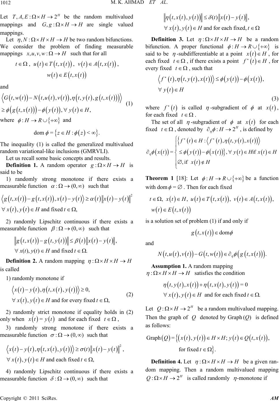


 .

1012 M. K. AHMAD ET AL.
Let ,, :2
H
TAE H 
,:Gg 
be the random multivalued
mappings and are single valued
mappings.
H H
Let ,:NHHH

 
,,,:
be two random bifunctions.
We consider the problem of finding measurable
mappings
x
uvw H such that for all
t, , ,
  
,ut Ttxt

,wt Et
  
,vt Atxt
 
xt
and
       

 

  
,,,,,,,
,, ,
GtwtNtut vttytgtxt
gtxtytyt H



 (1)
where and

:HR  

 
dom =:<.zH z  
The inequality (1) is called the generalized multivalued
random variational-like inclusions (GMRVLI).
Let us recall some basic concepts and results.
Definition 1. A random operator :
g
HH  is
said to be
1) randomly strong monotone if there exists a
measurable function :(0,)

 such that
      
 
2
,,,
, and fixed ,
g
txtgtxtxtyttxt yt
xt ytHt
 
 
2) randomly Lipschitz continuous if there exists a
measurable function :(0,)

 such that




 
,,
(),() and fixed .
,
g
txtgtytt xtyt
xt ytHt
 
 
Definition 2. A random mapping :
H
HH

 
is called
1) randomly monotone if
 
 
,,,0,
, and for every fixed ,
xtyttxtyt
xt ytHt
 
 
(2)
2) randomly strict monotone if equality holds in (2)
only when
 
=
x
tyt a n d for each fixed , t
3) randomly strong monotone if there exists a
measurable function :(0,)

 such that
    
 
2
,,,(),
, and each fixed ,
xt yttxtyttxt yt
xt ytHt
 
 

)
4) randomly Lipschitz continuous if there exists a
measurable function :(0,

 such that
 

  
 
,, (),
, and for each fixed,
txtytt xtyt
xt ytHt
 


Definition 3. Let :
H
HH


 be a random
bifunction. A proper functional


HR:  is
said to be

-subdifferentiable at a point

x
tH

, for
each fixed t

, if there exists a point

f
tH

, for
every fixed t

, such that
 

    

,, ,,
f
ttyt xtytxt
yt H
 


(3)
where


f
t
 is called

-subgradient of

at


x
t,
for each fixed t

.
The set of all

-subgradient of

at

x
t for each
fixed t

, denoted by :2
H
H

 , is defined by


 






 

:,,,
=, i
, if
ft Hfttytxt
f
x
tytxtytHxt
xtH





H

 






Theorem 1 [18]: Let be a function
with dom

:HR  
=


. Then for each fixed



  




 

, , ,, ,,
,
txtH utTtxtvtAtxt
wt Etxt
 

is a solution set of problem (1) if and only if




,dogtxt m


and
 

 

  

,,, ,Ntut vtGtwtgtxt

  .
Assumption 1. A random mapping
:
H
HH


 satisfies the condition






 


 
,,,,=0
, and for each fixed .
tyt xttxtyt
xt ytHt
 


2
Let :
H
QH 
Q
be a random multivalued mapping.
Then the graph of denoted by Graph is defined
as follows:
()Q
 


 



Graph = ,; ,,
for fixed .
QxtytHHytQtxt
t
 

Definition 4. Let :
H
HH


 be a given ran-
dom mapping. Then a random multivalued mapping
:2
H
QH  is called randomly

-monotone if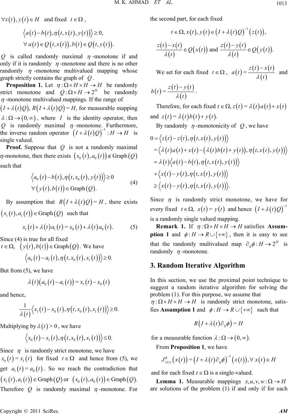

M. K. AHMAD ET AL.
1013
 
,
x
tytH and fixed t

,
  
     
,,,0,
,, ,
atbttxt yt
atQtxt btQtyt
 
 .
Q is called randomly maximal

-monotone if and
only if it is randomly

-monotone and there is no other
randomly

-monotone multivalued mapping whose
graph strictly contains the graph of . Q
Proposition 1. Let :
H
HH


:2
 be randomly
strict monotone and
H
QH be randomly

-monotone multivalued mappings. If the range of




I
tQ  ,
 
=RI tQ
H
 , for measurable mapping

:0,   

, where
I
is the identity operator, then
is randomly maximal Q

-monotone. Furthermore,
the inverse random operator


1:
I
tQH H 

 is
single value d.
Proof. Suppose that is not a randomly maximal
Q

-monotone, then there exists
 




00
,Graph
x
tat Q

such that
  
   
00
,,, 0
,Graph.
at bttxtyt
yt btQ
 
 (4)
By assumption that , there exists
 
=RItQ H  

aph
  
11
,Gr
x
tatQ
such that
 


110 0
= .
x
ttatxttat  
(5)
Since (4) is true for all fixed
. We have ,t
   
, Graphyt btQ
  
01 01
,,, 0at attxtxt  .
But from (5), we have
   
01 10
= tatatxtxt  
and hence,
  

10 01
1,,, 0.
xt xttxt xt
t



Multiplying by, we have

>0t 
  
01 01
,,, 0xt xttxtxt  .
Since

is randomly strict monotone, we have




01
=
x
txt
for fixed t and hence from (5), we 
get . So we reach the contradiction that
 
10
=at at
   

11
,Graph
x
tatQ
or
 




00
,Graph
x
tat Q.
Therefore is randomly maximal
Q

-monotone. For
the second part, for each fixed
    
1
, ,,txtytItQzt 

 




 

and
zt xtQxt
t 

 
 

zt ytQyt
t

.
t
We set for each fixed

,
 



=zt xt at t

 and






=zt yt bt t

.
Therefore, for each fixed
 




, =tzt tatx   t
and








=
z
ttbty  t
.
By randomly

-monotonicity of , we have Q








     
  
 
 
0,,,
= ,,,
,, ,
,, ,
,, ,.
ztzttxtyt
tatxttbtyttxt yt
tatbttxtyt
xtyttxt yt
xtyttxt yt










Since

is randomly strict monotone, we have for
every fixed t

,




=
x
tyt and hence
 
1
I
tQ 


is a randomly single valued mapping.
Remark 1. If :
H
HH


 satisfies Assum-
ption 1 and


:HR   , then it is easy to see
that the randomly multivalued map :2
H
H

  is
randomly

-monotone.
3. Random Iterative Algorithm
In this section, we use the proximal point technique to
suggest a random iterative algorithm for solving the
problem (1). For this purpose, we assume that
:
H
HH


 is randomly strict monotone, satis-
fies Assumpti on 1 and such that

:HR  




=RI tH

 

forameasurablefunction :0,.  
From Prop o si tion 1, we have
  


  
1
() =,
t
J
xtItxtxtH






andforeachfixed t

is a single-valued.
Lemma 1. Measurable mappings ,,,:
x
uvw H


are solutions of the problem (1) if and only if for each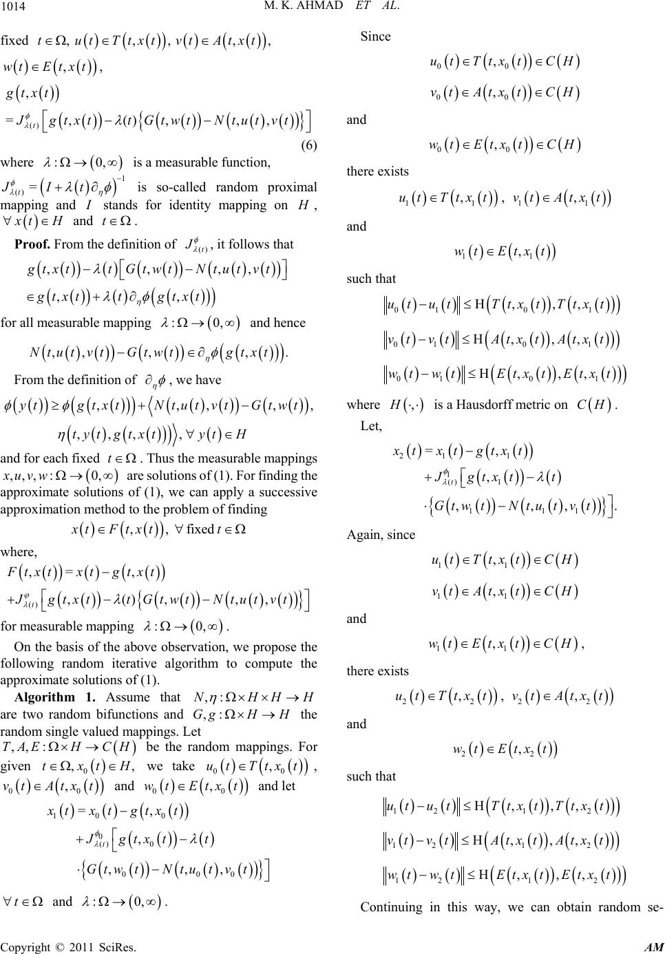

M. K. AHMAD ET AL.
1014


fixed
,
,t
, Etx
  
,,ut Ttxt
 
t
  
,,vtAtxt

wt
 





 
()
,
= , (),,,
t
gtxt
JgtxttGtwtNtutvt






(6)
where is a measurable function,

:0,  
 

1
JIt

() =
t





 is so-called random proximal
mapping and
I
stands for identity mapping on
H
,


x
tH and t.
Proof. From the definition of ()t
J


, it follows that
       


 
 
,,,
,,
,
g
txttGtwtNtut vt
gtxtt gtxt







for all measurable mapping and hence

:0,  

.
 




 
,, ,,Ntut vtGtwtgtxt

 
From the definition of


, we have
   

 






 
 

,,,,
,,,,
ytgtxtNtut vtGtwt
tyt gtxtytH


 

,

H
and for each fixed . Thus the measurable mappings
are solutions of (1). For finding the
approximate solutions of (1), we can apply a successive
approximation method to the problem of finding
t

,

,,,:0xuvw
  
,, fixed xt Ftxtt
where,
   
      

()
, = ,
,(), ,,
t
Ftxtxtgtxt
JgtxttGtwtNtutvt





 

for measurable mapping .

:0,   
On the basis of the above observation, we propose the
following random iterative algorithm to compute the
approximate solutions of (1).
Algorithm 1. Assume that ,:NHH

 
,:Gg H H are two random bifunctions and the
random single valued mappings. Let

,, :TAEH CH

0
, ,txtH 
be the random mappings. For
given we take





00
,ut Ttxt,





00
,vt Atxt and and let

0
wt E
 
0
,txt




  
    

10 0
0
() 0
000
= ,
,
,,,
t
xtxt gtxt
Jgtxtt
Gtw tNtutv t








 
t and .

:0,  
Since



 
00
,ut TtxtCH





00
,vt AtxtCH
and





00
,wt EtxtCH
there exists






11
,ut Ttxt,
 

11
,vt Atxt
and

 
11
,wt Etxt

such that
    


 


 
 


 
010 1
0101
010 1
H, ,,
H, ,,
H, ,,
utu tTtxtTtx t
vt vtAtxtAtxt
wt wtEtxtEtxt



where


,H

 is a Hausdorff metric on


CH.
Let,






  
    

21 1
1
() 1
111
= ,
,
,,,
t
xtxtgtxt
Jgtxt t
GtwtNtutv t








 .
Again, since



 
11
,ut TtxtCH



 
11
,vt AtxtCH
and



 
11
,wt EtxtCH,
there exists






22
,ut Ttxt,
  
22
,vt Atxt
and



22
,wt Etxt

such that
 





    

 


 
121 2
1212
1212
H, ,,
H, ,,
H, ,,
u tutTtx tTtxt
vt vtAtxtAtxt
w twtEtx tEtxt



Continuing in this way, we can obtain random se-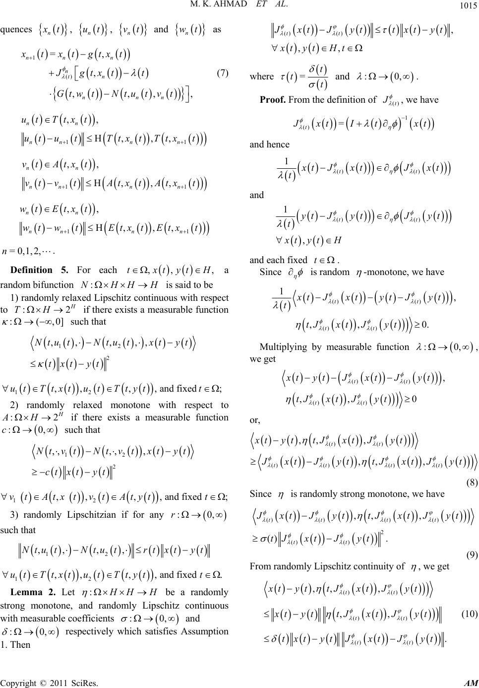

M. K. AHMAD ET AL.
1015
quences
 
n
x
t, ,
 
n
ut



n
vt and

 
n
wt

,
as
 




    

1
()
= ,
,
,,,
nn n
ntn
nnn
xtxt gtxt
Jgtxt t
Gtw tNtut vt








 
(7)
  
 




11
,,
H, ,,
nn
nnn n
ut Ttxt
ututTtxt Ttxt


 
  
    

11
,,
H, ,,
nn
nnnn
vt Atxt
vt vtAtxtAtxt



  
    

11
,,
H, ,,
nn
nnn n
wt Etxt
wt wtEtxt Etxt



=0,1,2, n.
Definition 5. For each a
random bifunction is said to be
 
,,txtytH 
HH 
,
2
:NH
1) randomly relaxed Lipschitz continuous with respect
to :
H
TH 
:(,0]  if there exists a measurable function
such that 
     
 
12
2
,, ,,, Ntu tNtutxtyt
txtyt 
 

 

 


12
,,,, andfixed ;u tTtxtutTtytt 
2
2) randomly relaxed monotone with respect to
:
H
AH

:0,c 
if there exists a measurable function
such that
     
 
12
2
,,,,, Nt vtNt vtxtyt
ct xtyt

 
 

 


12
,,,, andfixed vt Atxtvt Atytt ; 
3) randomly Lipschitzian if for any


:0,r
such that
     


12
,,,, Ntu tNtutrtxtyt
    


12
,,,, andfixed .utTtxtut Ttytt 
Lemma 2. Let :
H
HH

 
:  
be a randomly
strong monotone, and randomly Lipschitz continuous
with measurable coefficients and
respectively which satisfies Assumption
1. Then

0,


 

  
 
()() ,
,,
tt
J
xtJyttxtyt
xt ytHt


 

where




=t tt


and .

:0,   
Proof. From the definition of ()t
J


, we have
  


 
1
() = t
J
xtItxt





and hence
  


 

() ()
1tt
x
tJ xtJxt
t





and
  


 

 
() ()
1
,
tt
y
tJ ytJyt
t
xt ytH






and each fixed t

.
Since



is random

-monotone, we have
  

 
 
   

() ()
() ()
1,
,, 0.
tt
tt
x
tJ xtytJyt
t
tJxt Jyt








Multiplying by measurable function


:0,   ,
we get
 











() ()
() ()
,
,, 0
tt
tt
xtyt Jxt Jyt
tJxt Jyt





 

or,
 


 



       

() ()
()()() ()
,, ,
,,,
tt
tt tt
xtyttJxt Jyt
J
xtJ yttJxtJyt


 
 




(8)
Since

is rando mly strong monotone, we have


 

   



   
()()() ()
2
() ()
,, ,
() .
tt tt
tt
JxtJyt tJxtJyt
tJxt Jyt
 
 






(9)
From randomly Lipschitz continuity of

, we get
 

  


 




    
() ()
() ()
()()
,, ,
,,
.
tt
tt
tt
xtyttJxt Jyt
xtyttJxtJyt
txtytJxtJyt











 
(10)


:0,   

1016 M. K. AHMAD ET AL.
From (8)- ( 10 ), we have
 
 

()() ,
, where =.
tt
J
xtJytt xtyt
t
xt ytHtt







Definition 6. A random multivalued mapping

:
A
HCH

:0,   
is called randomly H-Lipschitz con-
tinuous if there exists a measurable function
such that
   

 
 
H,,,
,, and fixed .
,
A
txtAtytt xtyt
xt ytHt
 

Theorem 2. Let :
H
HH

  be a randomly
strong monotone and randomly Lipschitz continuous
with corresponding random coefficients


t  and
and satisfy the Assumption 1. Let

t 
,, :2
H
TAE H be the randomly H-Lipschitz con-
tinuous with corresponding random coefficients


,t 

t

and

t

respectively. Let ,:
g
GHH be
a randomly Lipschitz continuous with random coeffi-
cients


,t 

t 
NHH 
respectively and randomly strong
monotone with random coefficient. Let


t 
H: be a randomly relaxed Lipschitz
continuous with respect to random operator T with
random coefficients , randomly relaxed monotone
with respect to random operator

t 
A
with random
coefficient and randomly Lipschitz continuous
with respect to first and second arguments with random
coefficients

ct


rt and

s
t


respectively. For each n
let and be the
mappings such that

:
nHR
 

:  

HR





==
n
RI tRI tH

  
for .

>0t 
Assume that for fixed , t
    
1
()() = 0, for
lim nn
tt
n
J
ztJztzt H



 
(11)
If
  


  

  
 

 
 



 

2
22
2
2
22
(1 )
1
<
tctttt tpt
ttrttsttttt
tctttttptB
trttsttttt

 

 


 

where,
 

  

 

 

22
=
11,
Btrttstt ttt
tpt tpt
 


 
 

 

 
2
1
>tt ptB ct ttt












 
>,
<1, 1<, >,
rtt stttt
ptptt ctt



 (12)
 

 
2
=11 2.pttt t  
Then there exist, for any fixed , t


,
x
tH






,,ut Ttxt

 
,,vtAtxt





,Etxt
om varia-
wt
an

tio
satisfying the generalized multivalued rd
nal like inclusions (1) and




,t
n
ut u




,
n
v
tvt




,
n
wt wt
 
n
x
txt in
H
for
fixed t

,


n, where the random iterative
sequences




,
n
ut




n
vt ,
 
n
wt

and


n

x
t
are generated by random iterave Algorithm
of. Fr Algoritti 1.
Pro om hm 1, we have




 



     








 
 
 
    

   




1
1
1( ) 1
111
11
()
1
()
,,,
,,
,,,
,,
,,
,,
n
nnnn
n
ntn
nnn
nnn n
ntnn
n
nnt
xt
tGtwtNtutvtx t
gtx tJgtxtt
GtwtNtut vt
xtx tgtxtgtxt
JgtxttGtwt
Ntu t v tJg
















 


 


 
 








 


 


1n
xt

()
= ,,
nn tn
xt gtxtJ gtxt






 


 
 







    
 


 





 
   

 
1
111
11
1
1
11 ()1
1
() 11
1
,
,,,
,,
,, ,
,,,
,,
1
,,
n
nnn
nnn n
nn n
nnn
n
nn tn
ntnnn
nn nn
txt
tGtw tNtu tv t
xtx tgtxtgtxt
tgtxtgtxttGtwt
GtwtNtu t v t
NtutvtJ hxt
Jhxt txtxt
gtx tgtxttx tx













 





 
 








 


 

 
 
    
 

 

1
11
1
1
() 1()1
,,, ,
,,
nnn n
nn
nn
tnt n
t
tNtutvtN tutvt
tt GtwtGtwt
J hxtJhxt












(13)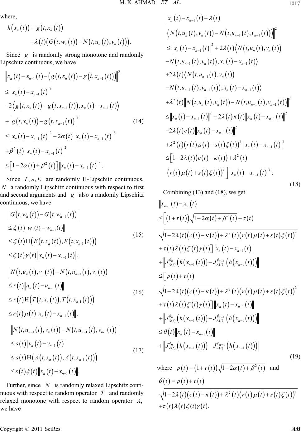

M. K. AHMAD ET AL.
1017
where,
.
Since
   
     

=,
,,,
nn
nnn
hx tgtx t
tGtwtNtutvt
 
g
is randomly strong monotone and randomly
Lipschitz continuous, we have
 


 
 




 
   
  
 
 
2
11
2
1
11
2
1
2
1
2
21
2
21
,,
2,, ,
,,
2
12.
nnn n
nn
nnnn
nn
nn nn
nn
nn
xtx tgtxtgtx t
xt xt
2
1
g
tx tgtxtxtxt
gtx tgtxt
xtx ttxtxt
txtxt
ttxtxt










 

 

 


 


(14)
Since are randomly H-Lipschitz continuous,
a ipschitz continuous with respect to first
and secoents and
,,TAE
randomly L
nd argum
N
g
also a rand omly Lip schitz
continuous, we have
   

    

 
1
1
-1
1
,,
()()
H, ,,
nn
nn
nn
nn
GtwtGtwt
twt w t
tEtx tEtxt
ttxtxt










,
(15)
 

 

 
    

 
1
1
,,, ,
H
nnn n
nn
NtutvtNtu tvt
rt utut



 (16)
-1
1
,,,
,
nn
nn
rt Ttx tTtxt
rtt x txt




 



 
 


 
 

11
1
-1
1
,, ,,
H, ,,
.
nn nn
nn
nn
nn
Ntutvt Ntutvt
st vtvt
stAtxtAtxt
sttx txt 







-1
(17)
Further, since is randomly relaxed Lipschitz conti-
nuous with resprandom operator and randomly
relaxed monotth respect to ran operator
N
ect to
one wiT dom ,
A






     

 

    
 
 

 
 

 

  
 
2
nn nn
nn
tctx tx



1
2
11
2
1
11
1
11 1
2
211
22
11
,,, ,
2,,
,,,
2,,
,, ,
,,, ,
2
nn
nnn n
nn nn
nnnn
nn
nn nn
nnnn
xt xtt
Ntu t v tNtut vt
xt xttNtutvt
Ntutvt xt xt
tNtutvt
Ntu tvtxtxt
tN tutvtN tutvt
xt xtttxt xt










 




 




 
 

 
2
1
22
2
t
trttsttxt xt 

 
   
    
1
2
22
12
.
nn
n
tc t tt
rttsttx txt





  





Combining (13) and (18), we get
1
n

(18)






 
  


we have
 
 

 


 



 
 






 
nn txt x  

1
2
2
1
1
() 1()1
2
2
1
1
() 1()1
112
12
12
nn
nn
nn
tnt n
nn
nn
tnt n
xtxt
tttt
tctttrtt
ttttxtxt
J hxtJhxt
pt t
tctttrtt s
ttttxtxt
J hxtJhxt



















 


 
 




 




2
st t


t t 

 

 
1
1
() 1()1
nn
tntn
t
J hxtJhxt






(19)
where
    
2
=112pttt t   and






  


 
2
2
=
12
() .
tptt
tctttrtt stt
tttt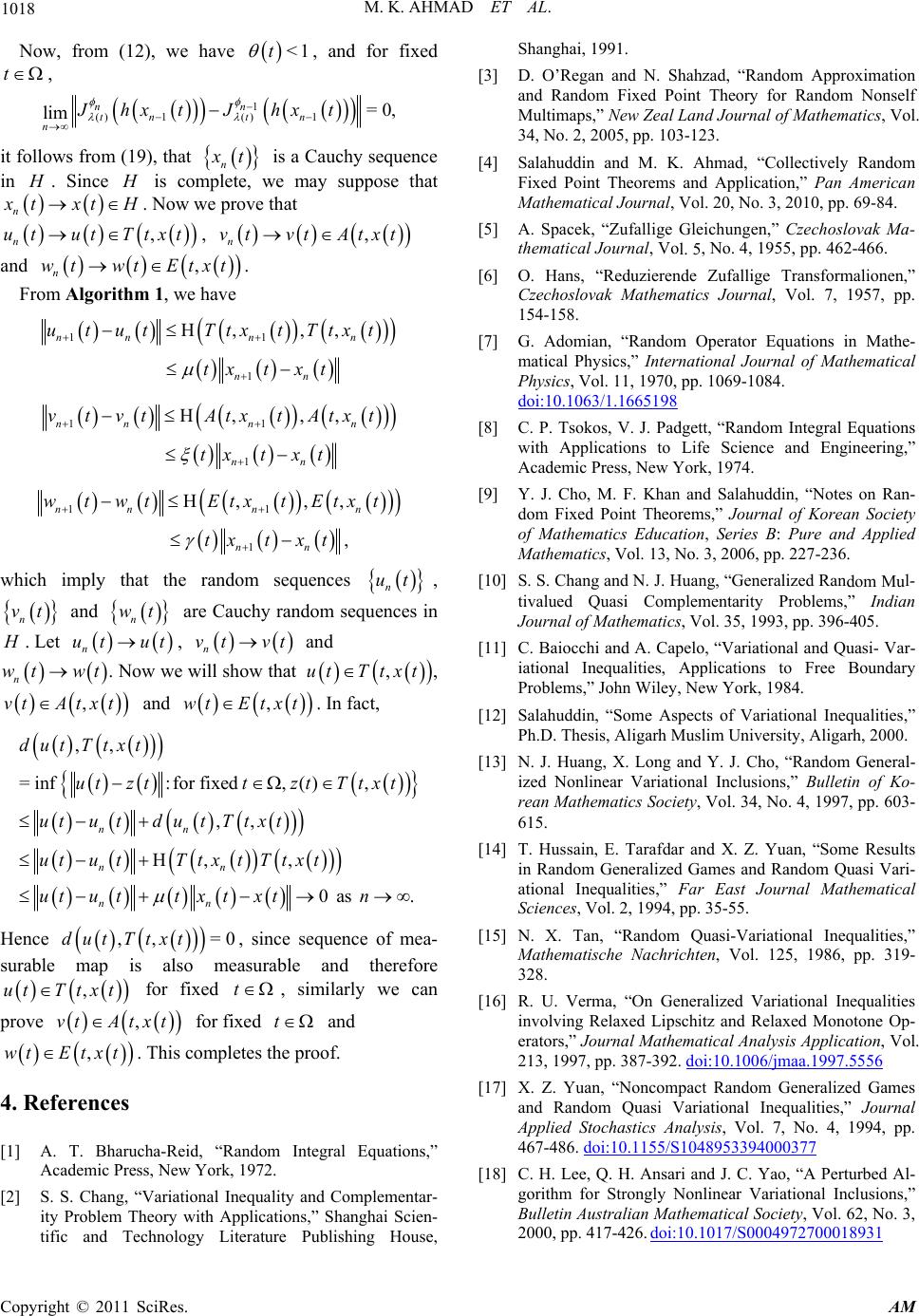




 


M. K. AHMAD ET AL.
1018
Now, from (12), we have and for fixed
,

<1t  ,
t
Shanghai, 1991.
 

 

1
()1()1 =0,
lim nn
tnt n
nJ hxtJhxt




 
it follows from (19), that



n
x
t is a Cauchy sequence
in
H
. Since
H
is coay suppose that mplete, we m
 
n
x
txt

nut
H
.
T
Nothat w we prove
,

ut
 
,txt



 
,vtAtxt
n
vt


,txt.
have
and

wt

wt
Algorithm 1
n
From
E
, we
  

 

 
11
1
H, ,,
nnn n
nn
utu tTtxtTtx t
txt xt 




 





 
11
1
H, ,,
nnnn
nn
vtvtAtxtAtxt
txt xt 




  

 


11
1
H, ,,
,
nnnn
nn
wtwt EtxtEtxt
txt xt 




wquences hich imply that the random se




n
ut
quences in
,
and are Cauchy random se


n
vt


n
wt
H
. Let

n
wt
 
ut
t. Now we
n
ut ,

w
 
n
vt vt
will show that
and





,Ttxt
fact,
ut,

. In

vt A


xt and ,t

,wt Etxt
 
 
  

 


    

 
,,
=inf : for fixed , (),
,,
H, ,
0 as .
nn
nn
nn
dutTtxt
utzttzt Ttxt
utu tdu tTtxt
ututTtx t Ttxt
utu tt xtxtn 

 
 
 
Hence 0, since sequence of mea-
surameasurable and therefore
  

,, =dutTtxt
ble map is also


,Ttxt for fixed t

ut


ed t
letes th
, similarly we can
and
f.
4. References
[1] A. T. Bharucha-Reid, “Random Integral Equations,”
Academic Press, New York, 1972.
[2] S. S. Chang, “Variational Inequality and Complemea
ity Problem Theory with Applications,” Shanghai Scien-
tific and Technology Literature Publishing House,
[3] D. O’Regan and N. Shahzad, “Random Approximation
and Random Fixed Point Theory for Random Nonself
Multimaps,” New Zeal Land Journal of Mathematicol.
34, No. 2, 2005, pp. 103-123.
. Ahma
F T
Mathematical 2010, pp. 69-84.
[5] A. Spacek, “Zufallige eichungen,” Czechoslovak Ma-
thematical Journal, Vo, No. 4, 1955, pp. 462-466.
O. Hans, “Reduzierende Zufallige Transformalionen,”
urnal, Vol. 7, 1957, pp.
154-158.
[7] G. Adomian, “Random Operator Equations in Mathe-
matical Physics,” International Journal of Mathematical
Physics, Vol. 11, 1970, pp. 1069-1084.
doi:10.1063/1.1665198
prove

wt
 

,vt Atxt for fix


,Etxt . This comp

e proo
s, V
[4] Salahuddin and M. Kd, “Collectively Random
ixed Pointheorems and Application,” Pan American
Journal, Vol. 20, No. 3,
Gl
l. 5
[6] Czechoslovak Mathematics Jo
[8] C. P. Tsokos, V. J. Padgett, “Random Integral Equations
with Applications to Life Science and Engineering,”
Academic Press, New York, 1974.
[9] Y. J. Cho, M. F. Khan and Salahuddin, “Notes on Ran-
dom Fixed Point Theorems,” Journal of Korean Society
of Mathematics Education, Series B: Pure and Applied
Mathematics, Vol. 13, No. 3, 2006, pp. 227-236.
dom Mu
tiv
Journal of Mathem
[11 aiocchi and A. Capelo, “Variati Quasi- Var-
iational o Free Boundar
Problems,” John Wileyrk, 1984
[12] Salahuddin, “Some Aspects of Variatiities,”
Ph.D. Thesis, Aligarh Muslim University, Aligarh, 2000.
[13] N. J. Huang, X. Long and Y. J. Cho, “Random General-
ized Nonlinear Variational Inclusions,” Bulletin of Ko-
rean Mathematics Society, Vol. 34, No. 4, 1997, pp. 603-
615.
[14] T. Hussain, E. Tarafdar and X. Z. Yuan, “Some Results
in Random Generalized Games and Random Quasi Vari-
ational Inequalities,” Far East Journal Mathematical
Sciences, Vol. 2, 1994, pp. 35-55.
[16] R. U. Vermalized
volving Relaxed Ltone Op-
erators,” Jour lication, Vol.
213, 1997, pp97.5556
[10] S. S. Chang and N. J. Huang, “Generalized Ranl-
alued Quasi Complementarity Problems,” Indian
atics, Vol. 35, 1993, pp. 396-405.
] C. Bonal and
Inequalities, Applications ty
, New Yo.
onal Inequal
[15] N. X. Tan, “Random Quasi-Variational Inequalities,”
Mathematische Nachrichten, Vol. 125, 1986, pp. 319-
328.
, “On GeneraVariational Inequalities
in ipschitz and Relaxed Mono
nal Mathematical Analysis App
. 387-392. doi:10.1006/jmaa.19
Noncompact Random Generalized Games
Quasi Variational Inequalities,” Journal
Applied Stochastics Analysis, Vol. 7, No. 4, 1994, pp.
[17] X. Z. Yuan, “
and Random
467-486. doi:10.1155/S1048953394000377
[18] C. H. Lee, Q. H. Ansari and J. C. Yao, “A Perturbed Al-
gorithm for Strongly Nonlinear Variational Inclusions,”
Bulletin Australian Mathematical Society, Vol. 62, No. 3,
2000, pp. 417-426. doi:10.1017/S0004972700018931
nt r-