J. Service Scie nce & Management, 2009, 3: 215-220
doi:10.4236/jssm.2009.23026 Published Online September 2009 (www.SciRP.org/journal/jssm)
A Quantity Discount Pricing Model Based on the
Standard Container under Asymmetric Information
Zhengping DING, Keyi WANG
School of Management, Dalian University of Technology, Dalian, China.
Received March 13th, 2009; revised April 29th, 2009; accepted June 1st, 2009.
ABSTRACT
A supply chain system is studied, in which the informatio n about the retailer’s storage cost is usually asymmetric. This
paper studies the inventory control in the system and presents a quantity discount pricing model for inventory coordi-
nation based on the standard container, a transport tool from the supplier to the retailer with a fixed size. First, it in-
vestigates the inventory mod els under full information. Before inventory co ordination, the supplier and the retailer my-
opically choose their lot sizes, which is not the optimal decision for the whole system. Then, it presents an incentive
scheme under asymmetric information from the point of view of the supplier. It also discusses the solution and the dis-
tribution of the incremental profits after the incentive scheme is adopted by both the supplier and the retailer. A con-
stant in the model, which affects the distribution of the incremental profits, is optimized for the supplier by using nu-
merical analysis. Finally, an example illustrates the application of the model. After inventory coordination, both the
supplier and the retailer have a positive in cremental profit.
Keywords: inventory coordin ation, asymmetric information, quantity discounts, standard container
1. Introduction
In order to improve managerial effectiveness, people
have traditionally focused their efforts on making effec-
tive decisions within an organization. Since the 1980s,
the supply chain management has become people’s focus.
A supply chain is a very complicated system; therefore,
coordination is the key point of the supply chain man-
agement.
Thomas & Griffin classifies supply chain coordination
into strategic coordination and operational coordination
[1]. In terms of operational coordination, the quantity
discount pricing model is a basic method of coordinating
in the supply chain, both in study and in practice.
Traditionally, quantity discount pricing models have
been studied from the point of view of the buyer, which
focus on the problem of determining the economic order
quantities for the buyer, given a quantity d iscount sched-
ule set by the supplier [2]. Goyal, one of the first schol-
ars studying the buyer-vendor inventory coordination
proposes an integrated inventory model from both the
point of view of the buyer and supplier [3]. Monahan
proposes a quantity discount pricing model to increase
the supplier profits [4]. Lee & Rosenblatt relax the im-
plicit assumption of a lot-for-lot policy adopted by the
supplier in Monahan’s model [2]. Weng studies the
all-unit quantity discount and the incremental quantity
discount, and shows that both these discounts are equi-
valent in achieving channel coordination [5].
Those traditional qu antity discount models are studied
under full information, and both the supplier and the
buyer exactly know the cost structure of each other.
However, in practice, such full information assumption
is very hard to satisfy [6,7]. Corbett & Groote propose a
quantity discount policy under asymmetric information
and compare it with the model under full information [6].
Guo Min & Wang Hongwei present a quantity discount
mechanism for the cooperation and coordination between
the two sides. The mechanism can make the buyer share
its information about storage holding cost with the sup-
plier [7].
On the other hand, quan tity discounts are often related
to transport tools in practice. Usually, the transport tools
are containers with standard sizes, and any lot size ad-
justment may force the buyer to carry less-than-truck
loads, resulting in hidden freight costs that were no t con-

ZHENGPING DING, KEYI WANG 216
sidered [8]. Pantumsinchai & Knowles propose algo-
rithms for solving an SPP in which Q is made up of a
number of containers with standard sizes. The news-
vendor can choose any combination of container sizes
and the larger the container, th e smaller the unit cost [9].
Shin & Benton consider that the lot-size should be aug-
mented by an integer multiple, and propose a quantity
discount approach to coordination [10]. But these re-
searches are all assumed that the supplier has full infor-
mation.
2*
21 2
23*
111
d() 20
dS
YNK QDS
KKkQ


In this paper, we study a supply chain system with a
standard transport tool under asymmetric information. In
the system, there are a single supplier and a single re-
tailer, and the transport too ls are standard containers with
same size. The supplier places quantity discount scheme
under asymmetric information about the retailer’s stor-
age cost, and the retailer chooses the lot-size according
to the scheme.
The study is based on the following assumptions. First,
the exogenous demand is constant and continuous. Sec-
ond, the supplement lead time is determinate. Third, no
shortages are allowed. The main symbols are listed as
follows:
D: the annual demand;
P: the retailer’s selling price;
P1: the retailer’s purchase price;
P2: the supplier’s purchase price;
h1: the retailer’s yearly unit holding cost;
h2: the supplier’s yearly unit holding cost;
S1: the retailer’s fixed ordering cost per order;
S2: the supplier’s fixed ordering cost per order;
QS: the size of the standard container;
Q: the retailer’s lot-size;
d: the unit discount under full information;
dA: the unit discount under asymmetric in formation;
YN1: the retailer’s yearly profit without discount;
YN2: the supplier’s yearly profit without discount;
YND1: the retailer’s yearly profit with discount;
YND2: the supplier’s yearly profit with discount.
2. The Inventory Model under Full
Information
2.1 The Inventory Model with Independent
Decision
Before coordination, both the supplier and the retailer
myopically choose the optimal lot-size according to their
own cost structure. The retailer’s yearly profit is
111
() ()//2YNQDPPDSQhQ
1

 ,
and the optimal lot-size is11
2/QDSh. Since the trans-
port tools are standard containers with same size, the
order should be transported with full container for eco-
nomic purpose. If Q isn’t an integ er multiple of the stan-
dard size, i.e., 1
s
QkQ

the retailer will compare the two
integer multiples of the standard size directly above and
below of Q to determine the optimal lot-size **
1
s
QkQ

to maximize his yearly profit.
Lee & Rosenblatt [2] show that, when the retailer’s
lot-size is, the supplier’s optimal lot-size
should be
**
1S
QkQ
11
**
1S
K
QKkQ

(K2
2
)
)
)
1 is a positive integer), and
the supplier’s average storage is . Then
the supplier’s yearly profit is
*
11
(1) /
S
KkQ
**
211 22 11
()( )/S YNK QDPPDSKkQ
*
21 1
(1)/
S
hK kQ
Since the second derivative of with re-
spect to K1 is
*
21
(YNKQ
there is a maximum of . So the parameter K1
could be derived by taking the first derivative of
with respect to K1 and setting it to zero. K1
can be derived as:
*
21
(YNK Q
*
21
(YNK Q
2
1*
12
12
S
DS
KkQ h  (1)
If K1 isn’t an integer, it will compare the two integers
directly above and below of K1 to determine the factor
to maximize the supplier’s yearly profit. If K1 is an
integer, the supplier’s yearly profit will be
*
1
K
** *
211 22212
()=( )2S YNKQDPPDS hkQ h 2.
Thus, as the retailer’s lot-size increases, the supplier’s
yearly profit increases as well.
2.2 The Iintegrated Inventory Model
Based on the above discussion, we know that the sup-
plier hopes that the retailer chooses the largest possible
lot-size. On the other hand, it can be derived that
1will be decreased as the retailer’s lot-size Q in-
creases (where ). For the whole system,
the optimal lot-size can be derived as following.
()YN Q
**
1S
QQ kQ
When the retailer’s lot-size is 2Sand the supplier’s
optimal lot-size iskQ
22 S
K
kQ, the system’s yearly profit is:

ZHENGPING DING, KEYI WANG 217
122 22 12
122222
222
(1)
(,)=()+() ()22
SS
SS SS
SS
hkQh KkQ DS DS
YNkQKkQ YNkQ YNKkQDPPkQ KkQ

  (2)
Accordingly, the parameter K2 could be derived by tak-
ing the first derivative from (2) with respect to K2. So K2
can be derived as:
2
2
22
2 1
S
DS
KkQ h  (3)
If K2 is an integer, 2 ; otherwise,
*
2
KK


*
22
1 KK
or


*
22
1KK . Here, [K2] is the integer
part of K2.
The steps for solving above question are as follows.
First, choosing a positive integer k2 within the interv al of


1, S
D
Q. Second, adding the k2 into (3), and getting
*
2
K
to maximize the system’s yearly profit. Then,
spreading all over k2 and choosing the optimal lot-size
(kQ,
*
2S**
22 S
K
kQ) to maximize the total profit.
It is obvious that , and
*
2
kk*
1
****
)
S22 2 11
**
211
(, )(
()0
SS
S
YNYNk QK k QYNkQ
YNK k Q
 

Therefore there is a positive incremental profit in the
system. But is the retailer’s optimal lot-size for
his yearly profit. When the retailer’s lot-size increases
from to , its incremental profit will be:
*
1S
kQ
*
2
kQ
*
1S
kQ S
**
11211
**
11 12 11
**
12
()k Q()
=+ <0
22
SS
SS
SS
YNkQ
hk QhkQ DS DS
kQ kQ


YN YN (4)
Therefore, the inventory optimization with the inte-
grated decision will decrease the retailer’s benefit. In
order to make the retailer accept the optimal lot-size, it is
necessary to give the retailer a quantity discount to com-
pensate it. With the integrated decision, the system’s
total profit is augmented by YN

. If the divisions of th e
incremental profit between the retailer and the supplier
are

and 1

(where [0,1]

),, the unit quantity
discount amount will be 1
()dYNYND

 
)
.
3. The Inventory Model under Asymmetric
Information
3.1 The Model
It is known from (4) that, the bigger the retailer’s yearly
unit holding cost h1, the bigger the compensation given
to the retailer. Under asymmetric information, the re-
tailer could hide h1 in order to gain more ben efit. There-
fore, the supplier must devise a rational compensating
mechanism to make the retailer give the true information.
As the information is asymmetric, the retailer knows
h1, but the supplier doesn’t know it. In order to coordi-
nate, the supplier gives a quantity discount scheme ac-
cording to the forecast value 1 of h1. It gives the lot-
size of discount point (A1S
kh ) and the unit discount
(A1 ). The retailer decides the lot-size according to
the scheme. Since the optimal lot-size for the whole sys-
tem is2S, the supplier could devise the unit discount
as following (kk ):
ˆ
h
Q
*ˆ
()
*
1
ˆ
()h
ˆ
()dh
*
kQ *
A2

*
A12 1
A*
21
ˆˆ
() ()
ˆ
0(
S
S
dh QkhQ
dQkhQ





(5)
Before coordination, the retailer’s yearly profit
is 11 1S
Y1 111 ()( )2
SS
NkQDPPDSkQhkQ

 , and the sup-
plier’s yearly profit is
2111 221111SS2
()()(1) 2
S
YNK k QDPPDSKkQKkQh

 . After
coordination, the retailer’s yearly profit is
D1A1A1A1A
()( )
SS
YNkQDPPdDS kQhkQ 2
S
,
and the supplier’s yearly profit is
D2A A12A2A A
AA2
()( )
(1) 2
SS
S
YNKk QDPPdDSKk Q
KkQh


To make the retailer give the true h1, it needs to let
D1AS be the maximum at 11
. Calculating the
first derivative of YN with respect to h
1, and
setting it to 0 at
(YNk Q ))
ˆ
hh
D1 A
(
S
k Q
1
h
1
ˆ
h

, then
A1 A1
11A2S S
kQh dS
hhkQ D









or
A1 1
A
A
b
2S
S
kQh S
dkQ D


)
S
)
S
(6)
Here b is a cons tant. The su pplier can cho ose a certa in
constant b for a quantity discount scheme. Different b’s
result in different schemes. When the retailer accepts the
quantity discount scheme, the constant b doesn’t affect
the retailer giving the true h1.
Therefore, from the point of view of the supplier, we
can derive the inventory coordination model under
asymmetric information as follows:
D2A A
max ()
S
YNKk Q (7)
(8)
*
D1A1 1
() (
S
YNk QYNkQ
**
D2A A211
()(
S
YNKk QYNKk Q (9)
s.t.
where (8) is the condition for the retailer to accept the
scheme, and (9) is the condition for the supplier to accept it.
From (6), the quantity discount scheme can ensure the
retailer giving the true information. Hereafter we assume
that 11
ˆ
hh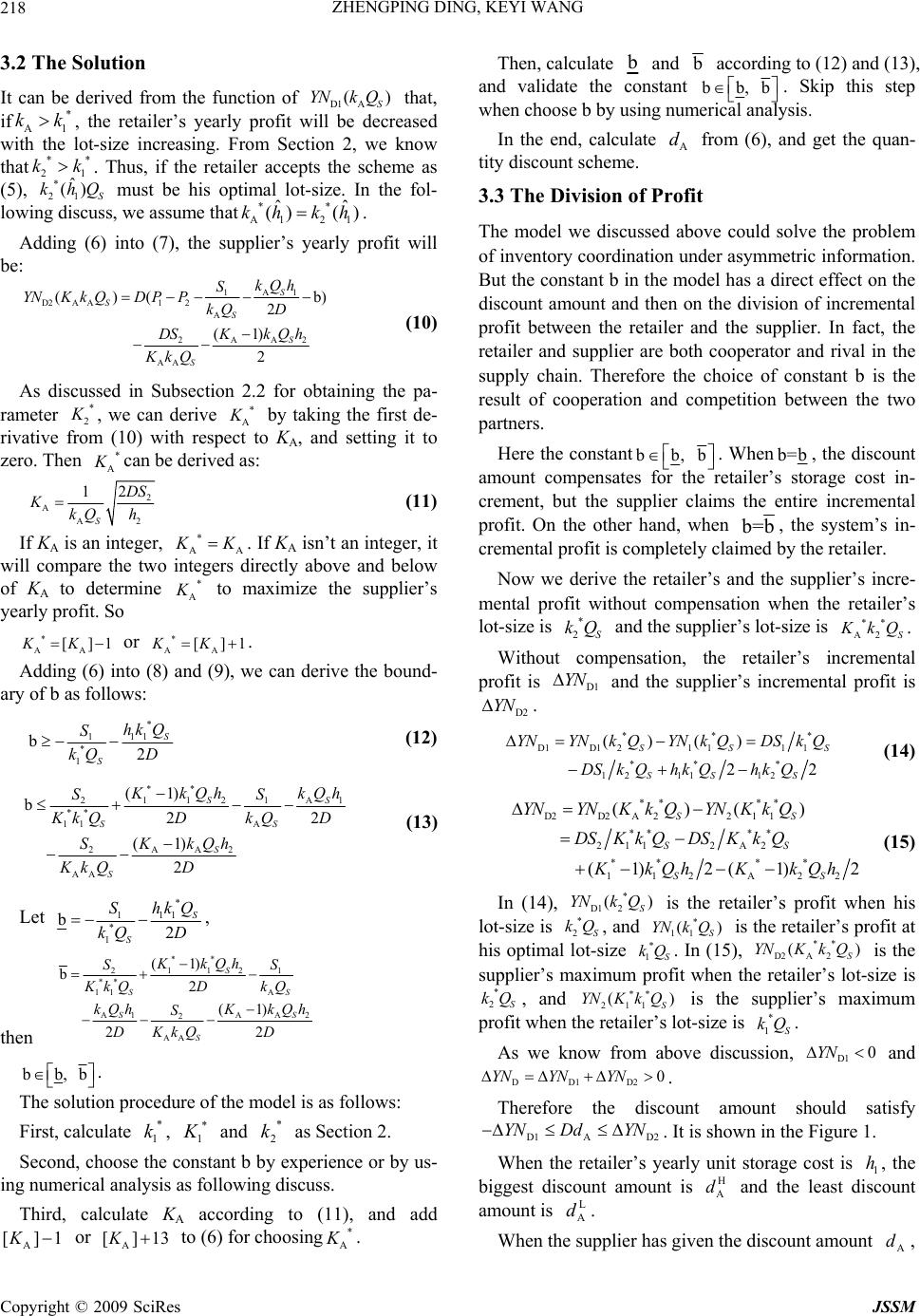

.

ZHENGPING DING, KEYI WANG 218
3.2 The Solution
It can be derived from the function of D1A that,
if , the retailer’s yearly profit will be decreased
with the lot-size increasing. From Section 2, we know
that . Thus, if the retailer accepts the scheme as
(5), S must be his optimal lot-size. In the fol-
lowing discuss, we assume that.
(
S
YNk Q
**
21
ˆˆ
()kh
)
*
*
A1
kk
*
2
k
*
21
ˆ
()kh
1
Q
k
A1
()kh
Adding (6) into (7), the supplier’s yearly profit will
be:
A11
()(b)
S
kQh S
YNKkQD PP 
D2 AA12
A
AA2 2
AA
2
(1
)
2
S
S
S
S
kQ D
KkQhDS
KkQ

 (10)
As discussed in Subsection 2.2 for obtaining the pa-
rameter *
2
K
, we can derive *
A
K
by taking the first de-
rivative from (10) with respect to KA, and setting it to
zero. Then *
A
K
can be derived as:
2
A
A2
2 1
S
D
S
KkQ h  (11)
If KA is an integer, A
*
A
K
K
*
A
. If KA isn’t an integer, it
will compare the two integers directly above and below
of K
A to determine
K
to maximize the supplier’s
yearly profit. So
*
AA
[]1KK
or .
*
AA
[]KK1
Adding (6) into (8) and (9), we can derive the bound-
ary of b as follows:
*
11 1
*
1
b2S
S
hkQ S
DkQ
  (12)
**
112A 21
** A11
AA2 2
AA
(1)
b22
(1)
2
SS
SS
S
S
KkQhkQh SS
DkQDKkQ
KkQh S
KkQD

 


1
(13)
Let *
hk Q S11
1
*
1
b2S
SDkQ
 ,
**
112
21
**
(1)
b2S
KkQh SS
DkQ KkQ

 
A 11
A1 A A2 2
AA
(1
)
22
S S
SS
S
kQhK kQh S
DKkQ D

 
then
b
b, b


.
The solution procedure of the model is as follows:
First, calculate ,
*
1
k*
1
K
and as Section 2.
*
2
k
Second, choose the constant b by experience or by us-
ing numerical analysis as following discuss.
Third, calculate KA according to (11), and add
or to (6) for choosing.
A
[]1KA []13K*
A
K
Then, calculate
b
and
b
according to (12) and (13),
and validate the constant
b
b, b
 .

Skip this step
when choose b by using numerical analysis.
In the end, calculate from (6), and get the quan-
tity discount scheme. A
d
3.3 The Division of Profit
The model we discussed above could solve the problem
of inventory co ordination under asymmetric information.
But the constant b in the model has a direct effect on the
discount amount and then on the division of incremental
profit between the retailer and the supplier. In fact, the
retailer and supplier are both cooperator and rival in the
supply chain. Therefore the choice of constant b is the
result of cooperation and competition between the two
partners.
Here the constant
b
b, b

 

. When
b
=b , the discount
amount compensates for the retailer’s storage cost in-
crement, but the supplier claims the entire incremental
profit. On the other hand, when
b
=b , the system’s in-
cremental profit is completely claimed by the retailer.
Now we derive the retailer’s and the supplier’s incre-
mental profit without compensation when the retailer’s
lot-size is and the supplier’s lot-size is
*
2S
kQ **
A2 S
K
kQ.
Without compensation, the retailer’s incremental
profit is D1
YN

and the supplier’s incremental profit is
D2
YN

.
** *
S
(
)
)
)
D1 D121 111
** *
12 1112
()()
22
SS
SS S
YNYNkQYNk QDSk Q
DSkQhkQhkQ
 
 (14)
15)
** **
D2D2A221 1
*** *
211 2A2
*** *
112A2
()()
(1)2( 1)
SS
SS
SS
YNYNKkQYNKk Q
DSK k QDSKkQ
KkQhK kQh


 
2
2
In (14), is the retailer’s profit when his
lot-size is 2S, and S is the retailer’s profit at
his optimal lot-size 1S. In (15), is the
supplier’s maximum profit when the retailer’s lot-size is
, and 21
1S
YN is the supplier’s maximum
profit when the retailer’s lot-size is .
*
D1 2
(
S
YNk Q
*
kQ YN
*
kQ
**
(Kk Q
*
11
(k Q
)
**
D2A 2
(
S
YNKkQ
*
1S
kQ
*
2S
kQ
As we know from above discussion, and
D1 0YN
DD1D2
0YN YNYN

 .
Therefore the discount amount should satisfy
D1 AD2
YN DdYN

. It is shown in the Figure 1.
When the retailer’s yearly unit storage cost is 1, the
biggest discount amount is and the least discount
amount is .
h
H
A
d
L
A
d
When the supplier has given the discount amount ,
A
d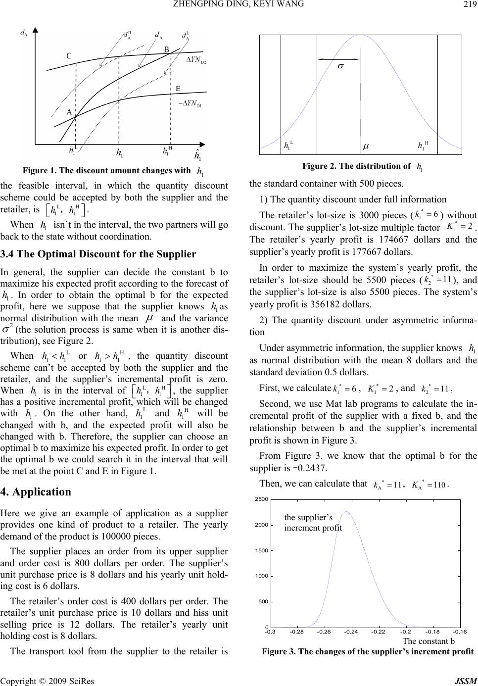

ZHENGPING DING, KEYI WANG 219
Figure 1. The discount amount changes with
1
h
the feasible interval, in which the quantity discount
scheme could be accepted by both the supplier and the
retailer, is .
LH
11
hh


，
h When 1 isn’t in the interval, the two partners will go
back to the state without coordination.
3.4 The Optimal Discount for the Supplier
In general, the supplier can decide the constant b to
maximize his expected profit according to the forecast of
1. In order to obtain the optimal b for the expected
profit, here we suppose that the supplier knows 1as
normal distribution with the mean
hh

and the variance
2

(the solution process is same when it is another dis-
tribution), see Figure 2.
When or , the quantity discount
scheme can’t be accepted by both the supplier and the
retailer, and the supplier’s incremental profit is zero.
When 1 is in the interval of 
, the supplier
has a positive incremental profit, which will be changed
with 1. On the other hand, and will be
changed with b, and the expected profit will also be
changed with b. Therefore, the supplier can choose an
optimal b to maximize his expected profit. In order to get
the optimal b we could search it in the interval that will
be met at the point C and E in Figure 1.
L
11
hhH
11
hh
h
h
LH
11
hh


，
L
1
h

H
1
h
4. Application
Here we give an example of application as a supplier
provides one kind of product to a retailer. The yearly
demand of the product is 100000 pieces.
The supplier places an order from its upper supplier
and order cost is 800 dollars per order. The supplier’s
unit purchase price is 8 dollars and his yearly unit hold-
ing cost is 6 dollars.
The retailer’s order cost is 400 dollars per order. The
retailer’s unit purchase price is 10 dollars and hiss unit
selling price is 12 dollars. The retailer’s yearly unit
holding cost is 8 dollars.
The transport tool from the supplier to the retailer is


L
1
hH
1
h
Figure 2. The distribution of
1
h
the standard container with 500 pieces.
1) The quantity di scount under full information
The retailer’s lot-size is 3000 pieces () without
discount. The supplier’s lot-size multiple factor
*
16k
*
12K

.
The retailer’s yearly profit is 174667 dollars and the
supplier’s yearly profit is 177667 dollars.
In order to maximize the system’s yearly profit, the
retailer’s lot-size should be 5500 pieces (*
211k

), and
the supplier’s lot-size is also 5500 pieces. The system’s
yearly profit is 356182 dollars.
2) The quantity discount under asymmetric informa-
tion
Under asymmetric information, the supplier knows 1
as normal distribution with the mean 8 dollars and the
standard deviation 0. 5 d ollars.
h
First, we calculate *
16k

, , and
*
12K* 211k

,
Second, we use Mat lab programs to calculate the in-
cremental profit of the supplier with a fixed b, and the
relationship between b and the supplier’s incremental
profit is shown in Figure 3.
From Figure 3, we know that the optimal b for the
supplier is -0.2437.
Then, we can calculate that , .
*
A11k*
A101K
Figure 3. The changes of the supplier’s increment profit
-0.3-0.28 -0.26-0.24 -0.22-0.2-0.18 -0.16
0
2 0
500
1 000
1 050
2 000
50
the supplier’s
increment profit
The constant b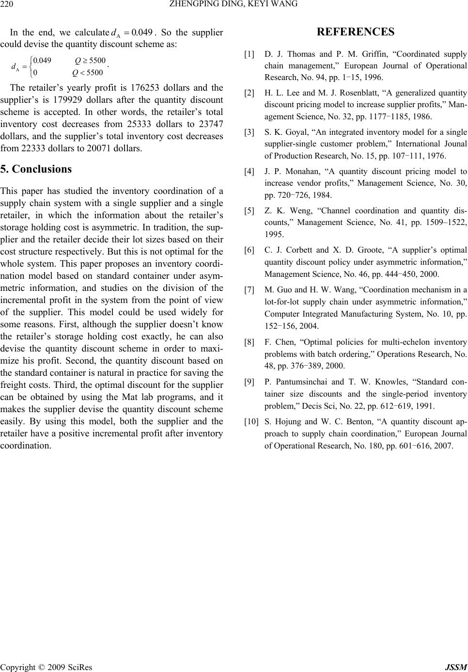

ZHENGPING DING, KEYI WANG 220
500
REFERENCES
In the end, we calculateA. So the supplier
could devise the quantity discount scheme as:
0.049d
[1] D. J. Thomas and P. M. Griffin, “Coordinated supply
chain management,” European Journal of Operational
Research, No. 94, pp. 1-15, 1996.
A
0.049 5500
05
Q
dQ



.
The retailer’s yearly profit is 176253 dollars and the
supplier’s is 179929 dollars after the quantity discount
scheme is accepted. In other words, the retailer’s total
inventory cost decreases from 25333 dollars to 23747
dollars, and the supplier’s total inventory cost decreases
from 22333 do llars to 200 71 dollars.
[2] H. L. Lee and M. J. Rosenblatt, “A generalized quantity
discount pricing model to increase supplier profits,” Man-
agement Science, No. 32, pp. 1177-1185, 1986.
[3] S. K. Goyal, “An integrated inventory model for a single
supplier-single customer problem,” International Jounal
of Production Research, No. 15, pp. 107-111, 1976.
5. Conclusions [4] J. P. Monahan, “A quantity discount pricing model to
increase vendor profits,” Management Science, No. 30,
pp. 720-726, 1984.
This paper has studied the inventory coordination of a
supply chain system with a single supplier and a single
retailer, in which the information about the retailer’s
storage holding cost is asymmetric. In tradition, the sup-
plier and the retailer decide their lot sizes based on their
cost structure respectively. But this is not optimal for the
whole system. This paper proposes an inventory coordi-
nation model based on standard container under asym-
metric information, and studies on the division of the
incremental profit in the system from the point of view
of the supplier. This model could be used widely for
some reasons. First, although the supplier doesn’t know
the retailer’s storage holding cost exactly, he can also
devise the quantity discount scheme in order to maxi-
mize his profit. Second, the quantity discount based on
the standard container is natural in practice for saving the
freight costs. Th ird, the optimal discount for the supp lier
can be obtained by using the Mat lab programs, and it
makes the supplier devise the quantity discount scheme
easily. By using this model, both the supplier and the
retailer have a positive incremental profit after inventory
coordination.
[5] Z. K. Weng, “Channel coordination and quantity dis-
counts,” Management Science, No. 41, pp. 1509–1522,
1995.
[6] C. J. Corbett and X. D. Groote, “A supplier’s optimal
quantity discount policy under asymmetric information,”
Management Science, No. 46, pp. 444-450, 2000.
[7] M. Guo and H. W. Wang, “Coordination mechanism in a
lot-for-lot supply chain under asymmetric information,”
Computer Integrated Manufacturing System, No. 10, pp.
152-156, 2004.
[8] F. Chen, “Optimal policies for multi-echelon inventory
problems with batch ordering,” Operations Research, No.
48, pp. 376-389, 2000.
[9] P. Pantumsinchai and T. W. Knowles, “Standard con-
tainer size discounts and the single-period inventory
problem,” Decis Sci, No. 22, pp. 612-619, 1991.
[10] S. Hojung and W. C. Benton, “A quantity discount ap-
proach to supply chain coordination,” European Journal
of Operational Research, No. 180, pp. 601-616, 2007.