Journal of Intelligent Learning Systems and Applications, 2011, 3, 171-180
doi:10.4236/jilsa.2011.33018 Published Online August 2011 (http://www.scirp.org/journal/jilsa)
171
A Cross Entropy-Genetic Algorithm for
m-Machines No-Wait Job-Shop Scheduling
Problem
Budi Santosa, Muhammad Arif Budiman, Stefanus Eko Wiratno
Industrial Engineering, Institut Teknologi Sepuluh Nopember, Surabaya, Indonesia.
Received October 26th, 2010; revised January 26th, 2011; revised February 6th, 2011.
ABSTRACT
No-wait job-shop scheduling (NWJSS) problem is one of the classical scheduling problems that exist on many kinds of
industry with no-wait constraint, such as metal working, plastic, chemical, and food industries. Several methods have
been proposed to solve this problem, both exact (i.e. integer programming) and metaheuristic methods. Cross entropy
(CE), as a new metaheuristic, can be an alternative method to solve NWJSS problem. This method has been used in
combinatorial optimization, as well as multi-external optimization and rare-event simulation. On these problems, CE
implementation results an optimal value with less computational time in average. However, using original CE to solve
large scale NWJSS requires high computational time. Considering this shortcoming, this paper proposed a hybrid of
cross entropy with genetic algorithm (GA), called CEGA, on m-machines NWJSS. The results are compared with other
metaheuritics: Genetic Algorithm-Simulated Annealing (GASA) and hybrid tabu search. The results showed that CEGA
providing better or at least equal makespans in comparison with the other two methods.
Keywords: No-Wait Job Shop Scheduling, Cross Entropy, Genetic Algorithm, Combinatorial Optimization
1. Introduction
No-wait job-shop scheduling problem (NWJJS) is a
problem categorized to non-polynomial hard (NP-Hard)
problem, especially for m-machines [1]. In a typical job
shop problem, each job has its own unique operation
route. Because the continuity of operation in each job
must be kept to avoid operation reworking or job redoing,
the use of incorrect method for scheduling purpose may
make the makespan significantly longer. In addition, the
existance of no-wait constraint, e.g. on metal, plastic, and
food industries, made the problem even more complex.
Many researches have been using various methods to
solve NWJJS. Genetic Algorithm-Simulated Annealing
(GASA) [2] and Hybrid Tabu Search [3] are examples of
methods used to solve this problem. Several methods fail
to achieve the optimum solution, others succeed, but
with relatively long computational time.
Cross entropy method, as a relatively new metaheuris-
tic, has been widely used in broad applications, such as
combinatorial optimization, continuous optimization, noisy
optimization, and rare event simulation [4]. On these
problems, cross entropy can find optimal or near optimal
solution with less computational time. However, using
original CE to solve large scale NWJSS requires longer
computational time. This paper proposed a new algo-
rithm of hybridized cross entropy with genetic algorithm
(CEGA). The proposed method is also new in solving
NWJSS problem. Using the hybrid of CE and GA the
computational time can be reduced significantly while
maintaining better makespan.
2. Problem Overview
NWJSS is a specific job-shop scheduling problem in
which a constraint not to allow any waiting time between
two sequential processes for each job applies. This kind
of problem can be found in many industries with “no-
wait” constraint, such as steel processing, plastic Indus-
tries, and chemical-related industries (such as pharmacy
and food industries), also for semiconductor testing pur-
poses [1] and [5]. On such industries, if there’s any wait-
ing time exist between processes, it may cause a defect
on the product and would require it to be reworked with
a certain process. It may also cause a product failure,
means that we must redo all the processes for related job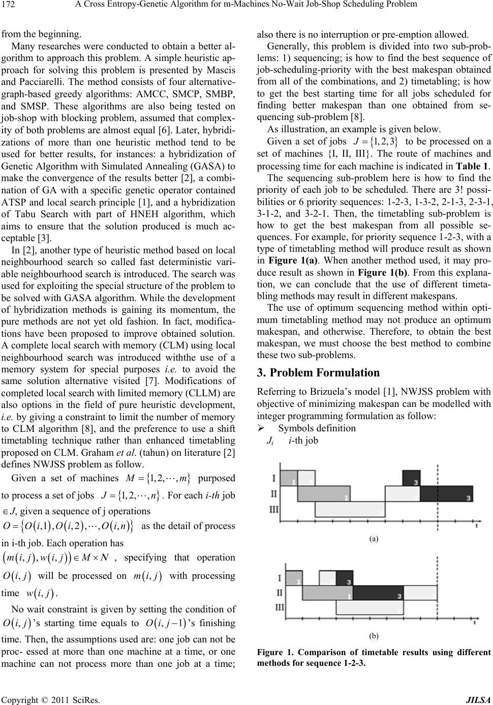

A Cross Entropy-Genetic Algorithm for m-Machines No-Wait Job-Shop Scheduling Problem 172
from the beginning.
Many researches were conducted to obtain a better al-
gorithm to approach this problem. A simple heuristic ap-
proach for solving this problem is presented by Mascis
and Pacciarelli. The method consists of four alternative-
graph-based greedy algorithms: AMCC, SMCP, SMBP,
and SMSP. These algorithms are also being tested on
job-shop with blocking problem, assumed that complex-
ity of both problems are almost equal [6]. Later, hybridi-
zations of more than one heuristic method tend to be
used for better results, for instances: a hybridization of
Genetic Algorithm with Simulated Annealing (GASA) to
make the convergence of the results better [2], a combi-
nation of GA with a specific genetic operator contained
ATSP and local search principle [1], and a hybridization
of Tabu Search with part of HNEH algorithm, which
aims to ensure that the solution produced is much ac-
ceptable [3].
In [2], another type of heuristic method based on local
neighbourhood search so called fast deterministic vari-
able neighbourhood search is introduced. The search was
used for exploiting the special structure of the problem to
be solved with GASA algorithm. While the development
of hybridization methods is gaining its momentum, the
pure methods are not yet old fashion. In fact, modifica-
tions have been proposed to improve obtained solution.
A complete local search with memory (CLM) using local
neighbourhood search was introduced withthe use of a
memory system for special purposes i.e. to avoid the
same solution alternative visited [7]. Modifications of
completed local search with limited memory (CLLM) are
also options in the field of pure heuristic development,
i.e. by giving a constraint to limit the number of memory
to CLM algorithm [8], and the preference to use a shift
timetabling technique rather than enhanced timetabling
proposed on CLM. Graham et al. (tahun) on literature [2]
defines NWJSS problem as follow.
Given a set of machines 
1, 2,,

M
m

1, 2,,
purposed
to process a set of jobs
J
n
 
in


, ,O

. For each i-th job
J, given a sequence of j operations
as the detail of process
in i-th job. Each operation has

 
,1,, 2,OOiOi


,, ,mij wijM



,j

,wij
, specifying that operation
will be processed on with processing
time .
Oi

,mij
No wait constraint is given by setting the condition of
’s starting time equals to ’s finishing
time. Then, the assumptions used are: one job can not be
proc- essed at more than one machine at a time, or one
machine can not process more than one job at a time;
also there is no interruption or pre-emption allowed.

,Oij
Generally, this problem is divided into two sub-prob-
lems: 1) sequencing; is how to find the best sequence of
job-scheduling-priority with the best makespan obtained
from all of the combinations, and 2) timetabling; is how
to get the best starting time for all jobs scheduled for
finding better makespan than one obtained from se-
quencing sub-problem [8].
As illustration, an example is given below.
Given a set of jobs


1, 2, 3J to be processed on a
set of machines {I, II, III}. The route of machines and
processing time for each machine is indicated in Table 1.
The sequencing sub-problem here is how to find the
priority of each job to be scheduled. There are 3! possi-
bilities or 6 priority sequences: 1-2-3, 1-3-2, 2-1-3, 2-3-1,
3-1-2, and 3-2-1. Then, the timetabling sub-problem is
how to get the best makespan from all possible se-
quences. For example, for priority sequence 1-2-3, with a
type of timetabling method will produce result as shown
in Figure 1(a). When another method used, it may pro-
duce result as shown in Figure 1(b). From this explana-
tion, we can conclude that the use of different timeta-
bling methods may result in different makespans.
The use of optimum sequencing method within opti-
mum timetabling method may not produce an optimum
makespan, and otherwise. Therefore, to obtain the best
makespan, we must choose the best method to combine
these two sub-problems.
3. Problem Formulation
Referring to Brizuela’s model [1], NWJSS problem with
objective of minimizing makespan can be modelled with
integer programming formulation as follow:
 Symbols definition
Ji i-th job
(a)
 
,1Oij
(b)
Figure 1. Comparison of timetable results using different
methods for sequence 1-2-3.
C opyright © 2011 SciRes. JILSA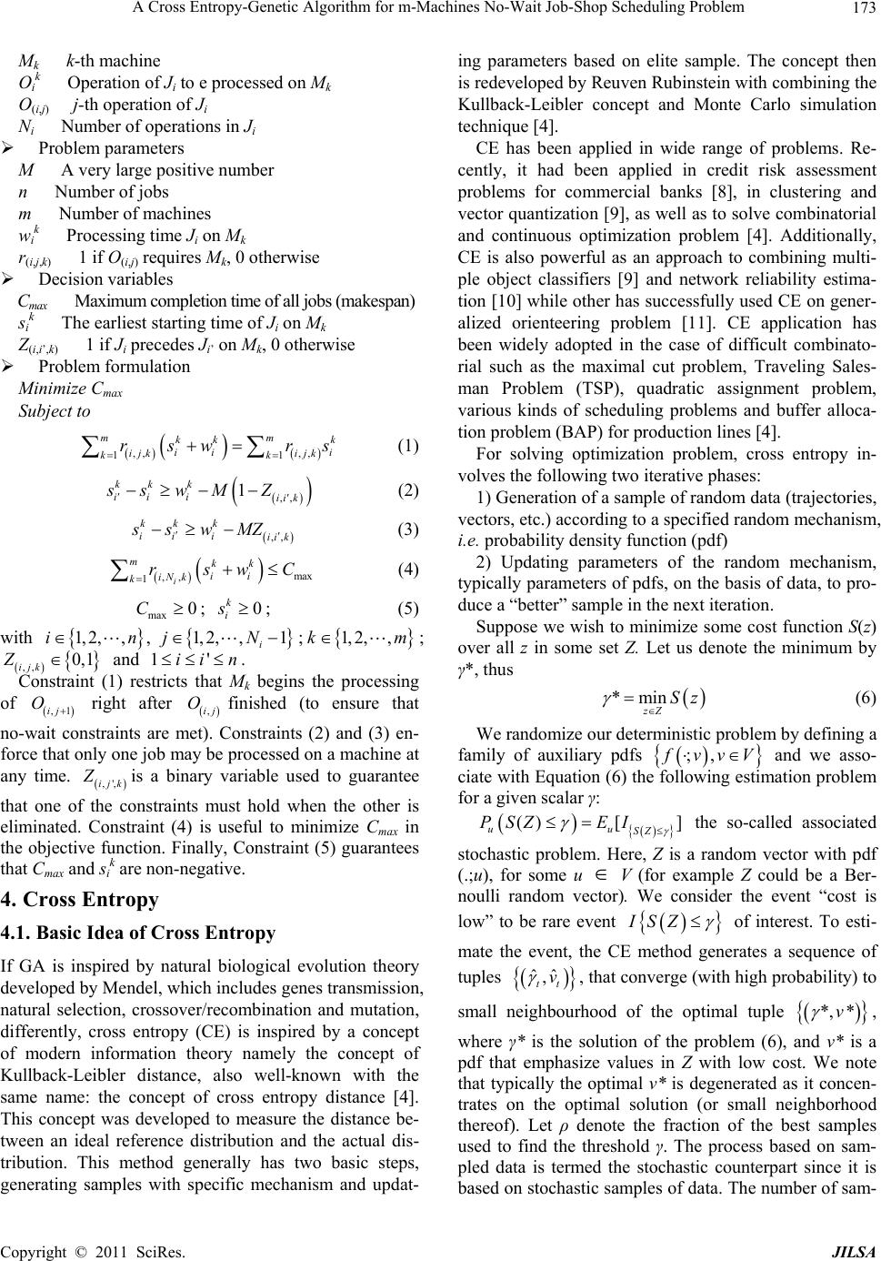

A Cross Entropy-Genetic Algorithm for m-Machines No-Wait Job-Shop Scheduling Problem173
m
k
k
Mk k-th machine
Oi
k Operation of Ji to e processed on Mk
O(i,j) j-th operation of Ji
Ni Number of operations in Ji
 Problem parameters
M A very large positive number
n Number of jobs
m Number of machines
wi
k Processing time Ji on Mk
r(i,j,k) 1 if O(i,j) requires Mk, 0 otherwise
 Decision variables
Cmax Maximum completion time of all jobs (makespan)
si
k The earliest starting time of Ji on Mk
Z(i,i’,k) 1 if Ji precedes Ji’ on Mk, 0 otherwise
 Problem formulation
Minimize Cmax
Subject to



,, ,,
11
m
kk
ii i
ijk ijk
k
rsw rs



(1)



,,
1
kk k
ii iii k
ss wMZ

  (2)

,,
kk k
ii iii k
ss wMZ

 


m

(3)


max
,,
1i
mkk
ii
iN k
krswC 
 (4)
max 0C; ; (5) 0
k
i
s
with ; ;
and .

1, 2,,,in


0, 1

1, 2,,1
i
jN
1'ii n 

1, 2,,k
,,ijk
Constraint (1) restricts that Mk begins the processing
of right after finished (to ensure that
no-wait constraints are met). Constraints (2) and (3) en-
force that only one job may be processed on a machine at
any time. is a binary variable used to guarantee
that one of the constraints must hold when the other is
eliminated. Constraint (4) is useful to minimize Cmax in
the objective function. Finally, Constraint (5) guarantees
that Cmax and si
k are non-negative.
Z

,1ij
O

,ij
O

,',ijk
Z
4. Cross Entropy
4.1. Basic Idea of Cross Entropy
If GA is inspired by natural biological evolution theory
developed by Mendel, which includes genes transmission,
natural selection, crossover/recombination and mutation,
differently, cross entropy (CE) is inspired by a concept
of modern information theory namely the concept of
Kullback-Leibler distance, also well-known with the
same name: the concept of cross entropy distance [4].
This concept was developed to measure the distance be-
tween an ideal reference distribution and the actual dis-
tribution. This method generally has two basic steps,
generating samples with specific mechanism and updat-
ing parameters based on elite sample. The concept then
is redeveloped by Reuven Rubinstein with combining the
Kullback-Leibler concept and Monte Carlo simulation
technique [4].
CE has been applied in wide range of problems. Re-
cently, it had been applied in credit risk assessment
problems for commercial banks [8], in clustering and
vector quantization [9], as well as to solve combinatorial
and continuous optimization problem [4]. Additionally,
CE is also powerful as an approach to combining multi-
ple object classifiers [9] and network reliability estima-
tion [10] while other has successfully used CE on gener-
alized orienteering problem [11]. CE application has
been widely adopted in the case of difficult combinato-
rial such as the maximal cut problem, Traveling Sales-
man Problem (TSP), quadratic assignment problem,
various kinds of scheduling problems and buffer alloca-
tion problem (BAP) for production lines [4].
For solving optimization problem, cross entropy in-
volves the following two iterative phases:
1) Generation of a sample of random data (trajectories,
vectors, etc.) according to a specified random mechanism,
i.e. probability density function (pdf)
2) Updating parameters of the random mechanism,
typically parameters of pdfs, on the basis of data, to pro-
duce a “better” sample in the next iteration.
Suppose we wish to minimize some cost function S(z)
over all z in some set Z. Let us denote the minimum by
γ*, thus

*min
zZSz


 (6)
We randomize our deterministic problem by defining a
family of auxiliary pdfs



;,
f
vvV and we asso-
ciate with Equation (6) the following estimation problem
for a given scalar γ:


 
()[ ]
uu
SZ
PSZ EI



 the so-called associated
stochastic problem. Here, Z is a random vector with pdf
(.;u), for some u

V (for example Z could be a Ber-
noulli random vector). We consider the event “cost is
low” to be rare event




ISZ

 of interest. To esti-
mate the event, the CE method generates a sequence of
tuples




ˆˆ
,
tt
v  , that converge (with high probability) to
small neighbourhood of the optimal tuple




*, *v  ,
where γ* is the solution of the problem (6), and v* is a
pdf that emphasize values in Z with low cost. We note
that typically the optimal v* is degenerated as it concen-
trates on the optimal solution (or small neighborhood
thereof). Let ρ denote the fraction of the best samples
used to find the threshold γ. The process based on sam-
pled data is termed the stochastic counterpart since it is
based on stochastic samples of data. The number of sam-

A Cross Entropy-Genetic Algorithm for m-Machines No-Wait Job-Shop Scheduling Problem 174
ples in each stage of the stochastic counterpart is denoted
by N, which is a predefined parameter. The following is
a standard CE procedure for minimization borrowed
from [4].
We initialize 00 and choose a not very small
ρ (rarity coeficient), say
ˆ
vvu
10 2

. We then proceed
iteratively as follows.
4.1.1. Adaptive updatin g o f γt
A simple estimator ˆt

of γt can be obtained by taking
random sample

1,
 
,
Z
ZN from the pdfs f(·;vt-1),
calculating the performance



lSZ for all l ordering
them from smallest to biggest as




1, ,SS
ˆt
N and
finally evaluating the ρ 100% sample percentile as


([ ])N
S

4.2.2. Adaptive updatin g o f vt
For a fixed γt and vt-1, derive vt from the solution of the
program:

 

1
minminln ;
tt
vSZ
vv
DvxEIf Zv




(7)
The stochastic counterpart of (7) is ˆt

and 1 ˆt v

, de-
rive from the following program:
ˆt v

 

()
1
1
ˆ
minminln ;
lt
Ni
SZ vv
l
DvIf Zv
N
 



(8)
The update formula of the kth element in v (Equation
(8)) in this case simply becomes:

 

 
1 ˆ
1
ˆ
1
ˆ
l lt
lt
N
Z SZ
i
tN
SZ
i
II
vk
I


 





(9)
To simplify Equation (9), we can use the following
smoothed version provided by [4]:

1
ˆˆ ˆ 1
tt t
vv v 

 (10)
where is the parameter vector obtained from the so-
lution of Equation (8), and β is a smoothing parameter.
The CE optimization algorithm is summarized in Algo-
rithm 1.
ˆt v
Algorithm 1. The CE Method for Stochastic Optimi-
zation
1) Choose . Set t = 1 (level counter)
0
2) Generate a sample Z(1),, Z(N) from the density f
(·;vt-1) and compute the sample ρ 100-percentile
ˆ
v
ˆt

of
the sample scores.
3) Use the same sample Z(1),, Z(N) and solve the
stochastic program (8). Denote the solution by .
t
v

4) Apply (10) to smooth out the vector .
t
v

ˆˆ
5) If for some , say d = 3, 1d dt ˆ
tt t




then stop; otherwise set t = t + 1 and reiterate from step
2.
It is found empirically that the CE method is robust
with respect to the choice of its parameter N, ρ, and β.
Typically those parameters satisfy that 0.01 0.1


,
0.5 0.9


, and , where n is the number of
parameter.
3Nn

This procedure provides the general frame. When we
are facing a specific problem, we have to modify it to fit
it with our problem.
4.2. Cross Entropy for Combinatorial
Optimization
In case of job scheduling we require parameter P in place
of v. P is a transition matrix where each entry pi,j denotes
the probability of the job i to the place j, for i = 1, 2,,
n, j = 1, 2,, n, where n is the number of job. For the
initial P we can put equal values to all entries, it means
that the probability of the job i to the place j is equally
distributed.
Based on matrix P, we will generate N sequences of
jobs. Each sequence (Zi) will be evaluated based on S(zi)
where S = Cmax value for each sequence. Out of N se-
quences, we take ρN percent elite samples with the best S
(instead of using  as a threshold to select elite sample).
Let ES = ρN, the updating formula for is given
by

ˆ,
t
Pij


1
ˆ,
ki
ES
Z
j
i
t
I
PijES


 (11)
To generate sequence of job we can use trajectory
generation using node placement [4] as shown in Algo-
ritm 1.
Algorithm 2. Trajectory generation using node place-
ment
1) Define P(1) = P, Let k = 1
2) Generate Zk from the distribution formed by the k-th
row of P(k). Obtain the matrix P(k+1) from P(k) by first
setting the Zk-th column of P(k) to 0 and then normalizing
the rows to sum up to 1.
3) If k = n then stop, otherwise k = k + 1 and reiterate
from Step 2.
4) Determine the sequences and evaluate their makespan
The main CE algorithm for job scheduling is given in
Algorithm 3.
Algorithm 3. The CE method for Job scheduling
1) Choose initial reference transition matrix 0, say
with all entries equal to 1/n, where n is the number of job.
Set t = 1.
ˆ
P
2) Generate a sample Z1, , ZN of job sequence via
Algorithm 2 with P = t-1 and choose ρN elite sample
with the best performance of S(z).

ˆ
P
3) Use the elite sample to update .
ˆt
P
4) Apply (10) to smooth out matrix .
ˆt
P
5) If for some , say d = 5, 1d tdˆˆ ˆ
tt t




then stop; otherwise set t = t+1 and reiterate from step 2.
4.3. Example
C opyright © 2011 SciRes. JILSA

A Cross Entropy-Genetic Algorithm for m-Machines No-Wait Job-Shop Scheduling Problem175
Table 1. NWJSS case example
Job Operation Machine Processing Time
1 O11 I 1
O
12 II 3
2 O21 I 1
O
22 II 4
O
23 III 2
3 O31 I 1
O
32 II 3
To understand the use of CE in jobshop scheduling more
easily, let’s see the following example. There are 3 jobs
with known processing time (L), due date (d) and weight
for tardiness (w) for each job as in Table 1. It is desired
to find the optimal sequence based on total weighted
tardiness. Let’s use N = 6, ρ = 1/3, β = 0.8.
The objective function for jobshop scheduling with
single machine with minimum total weighted tardiness
(SMTWT) is


1
minminmax, 0
n
zZkk k
k
Szwf d



where 1
n
kj
j
f
L


Suppose the initial transition matrix is
0
13 1313
13 1313
13 1313
P





and the population generated is as follows:
Z1: 1-2-3; with S = 1.5
Z2: 1-3-2; with S = 2
Z3: 2-1-3; with S = 0.5
Z4: 2-3-1; with S = 1
Z5: 3-1-2; with S = 2
Z6: 3-2-1; with S = 2
Two best samples as elite sample are
Z3: 2-1-3; with S = 0.5
Z4: 2-3-1; with S = 1
For the sequence 2−1−3, we have
0120
12 00
0012
w





Considering the second best sequence 2-3-1, we get
010
120 12
120 12
w





Using P1 = βw + (1 − β) P0, we obtain the transition
probability for the next iteration as
1
0.0667 0.8667 0.0667
0.4667 0.0667 0.4667
0.4667 0.0667 0.4667
P











Using this transition probability, N new sequences will
be generated. From these sequence, evaluate the objec-
tive function S(z) and repeat the same steps until stop-
ping criteria is met.
5. Proposed Algorithm
The proposed method to solve the NWJSS problem is a
hybrid of cross entropy with genetic algorithm (CEGA).
The cross entropy is used as the basic; while from the
GA the procedure of sample generation is adopted.
For this NWJSS problem, the flowchart of CEGA is
given in Figure 2.
The explanations of Figure 1 is as follows:
Defining Inputs and Outputs
The inputs and outputs are determined as follows:
Inputs:
 Machine routing matrix (R(j, k); j state the job number
and k state the operation number)
 Processing time matrix (W(j, k))
 Number of population (N)
 Ratio of elite sample (ρ)
 Smoothing coefficient (β)
 Initial crossover rate (Pps)
 Terminating criterion (  )
Figure 2. Flowchart of CEGA.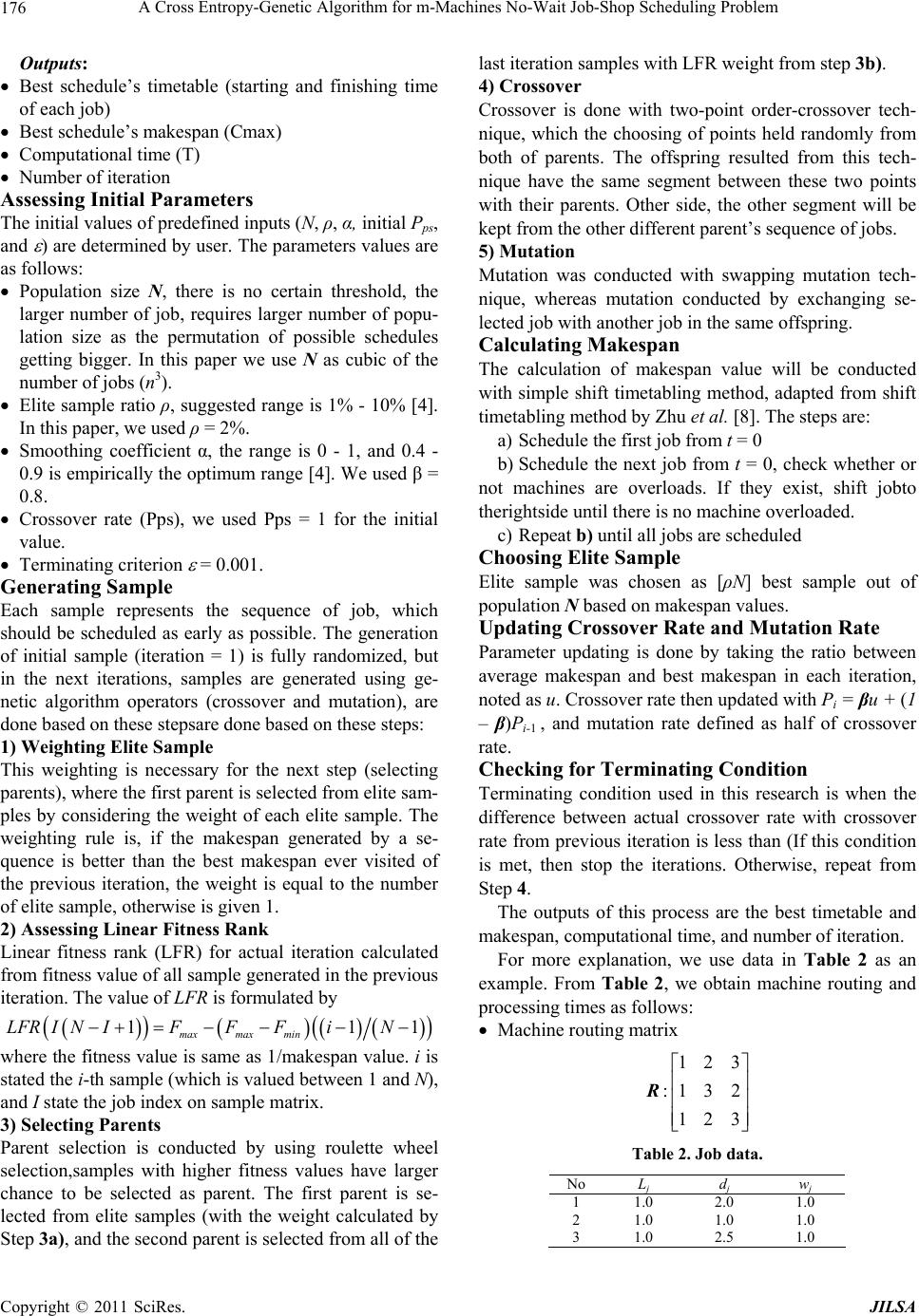

A Cross Entropy-Genetic Algorithm for m-Machines No-Wait Job-Shop Scheduling Problem 176
Outputs:
 Best schedule’s timetable (starting and finishing time
of each job)
 Best schedule’s makespan (Cmax)
 Computational time (T)
 Number of iteration
Assessing Initial Parameters
The initial values of predefined inputs (N, ρ, α, initial Pps,
and
 ) are determined by user. The parameters values are
as follows:
 Population size N, there is no certain threshold, the
larger number of job, requires larger number of popu-
lation size as the permutation of possible schedules
getting bigger. In this paper we use N as cubic of the
number of jobs (n3).
 Elite sample ratio ρ, suggested range is 1% - 10% [4].
In this paper, we used ρ = 2%.
 Smoothing coefficient α, the range is 0 - 1, and 0.4 -
0.9 is empirically the optimum range [4]. We used β =
0.8.
 Crossover rate (Pps), we used Pps = 1 for the initial
value.
 Terminating criterion  = 0.001.
Generating Sample
Each sample represents the sequence of job, which
should be scheduled as early as possible. The generation
of initial sample (iteration = 1) is fully randomized, but
in the next iterations, samples are generated using ge-
netic algorithm operators (crossover and mutation), are
done based on these stepsare done based on these steps:
1) Weighting Elite Sample
This weighting is necessary for the next step (selecting
parents), where the first parent is selected from elite sam-
ples by considering the weight of each elite sample. The
weighting rule is, if the makespan generated by a se-
quence is better than the best makespan ever visited of
the previous iteration, the weight is equal to the number
of elite sample, otherwise is given 1.
2) Assessing Linear Fitness Rank
Linear fitness rank (LFR) for actual iteration calculated
from fitness value of all sample generated in the previous
iteration. The value of LFR is formulated by
  

 
111
maxmax min
LFR INIFFFiN
where the fitness value is same as 1/makespan value. i is
stated the i-th sample (which is valued between 1 and N),
and I state the job index on sample matrix.
3) Selecting Parents
Parent selection is conducted by using roulette wheel
selection,samples with higher fitness values have larger
chance to be selected as parent. The first parent is se-
lected from elite samples (with the weight calculated by
Step 3a), and the second parent is selected from all of the
last iteration samples with LFR weight from step 3b).
4) Crossover
Crossover is done with two-point order-crossover tech-
nique, which the choosing of points held randomly from
both of parents. The offspring resulted from this tech-
nique have the same segment between these two points
with their parents. Other side, the other segment will be
kept from the other different parent’s sequence of jobs.
5) Mutation
Mutation was conducted with swapping mutation tech-
nique, whereas mutation conducted by exchanging se-
lected job with another job in the same offspring.
Calculating Makespan
The calculation of makespan value will be conducted
with simple shift timetabling method, adapted from shift
timetabling method by Zhu et al. [8]. The steps are:
a) Schedule the first job from t = 0
b) Schedule the next job from t = 0, check whether or
not machines are overloads. If they exist, shift jobto
therightside until there is no machine overloaded.
c) Repeat b) until all jobs are scheduled
Choosing Elite Sample
Elite sample was chosen as [ρN] best sample out of
population N based on makespan values.
Updating Crossover Rate and Mutation Rate
Parameter updating is done by taking the ratio between
average makespan and best makespan in each iteration,
noted as u. Crossover rate then updated with Pi = βu + (1
– β)Pi-1 , and mutation rate defined as half of crossover
rate.
Checking for Terminating Condition
Terminating condition used in this research is when the
difference between actual crossover rate with crossover
rate from previous iteration is less than (If this condition
is met, then stop the iterations. Otherwise, repeat from
Step 4.
The outputs of this process are the best timetable and
makespan, computational time, and number of iteration.
For more explanation, we use data in Table 2 as an
example. From Table 2, we obtain machine routing and
processing times as follows:
 Machine routing matrix
123
:1 32
123










R
Table 2. Job data.
No Lj d
j w j
1 1.0 2.0 1.0
2 1.0 1.0 1.0
3 1.0 2.5 1.0
C opyright © 2011 SciRes. JILSA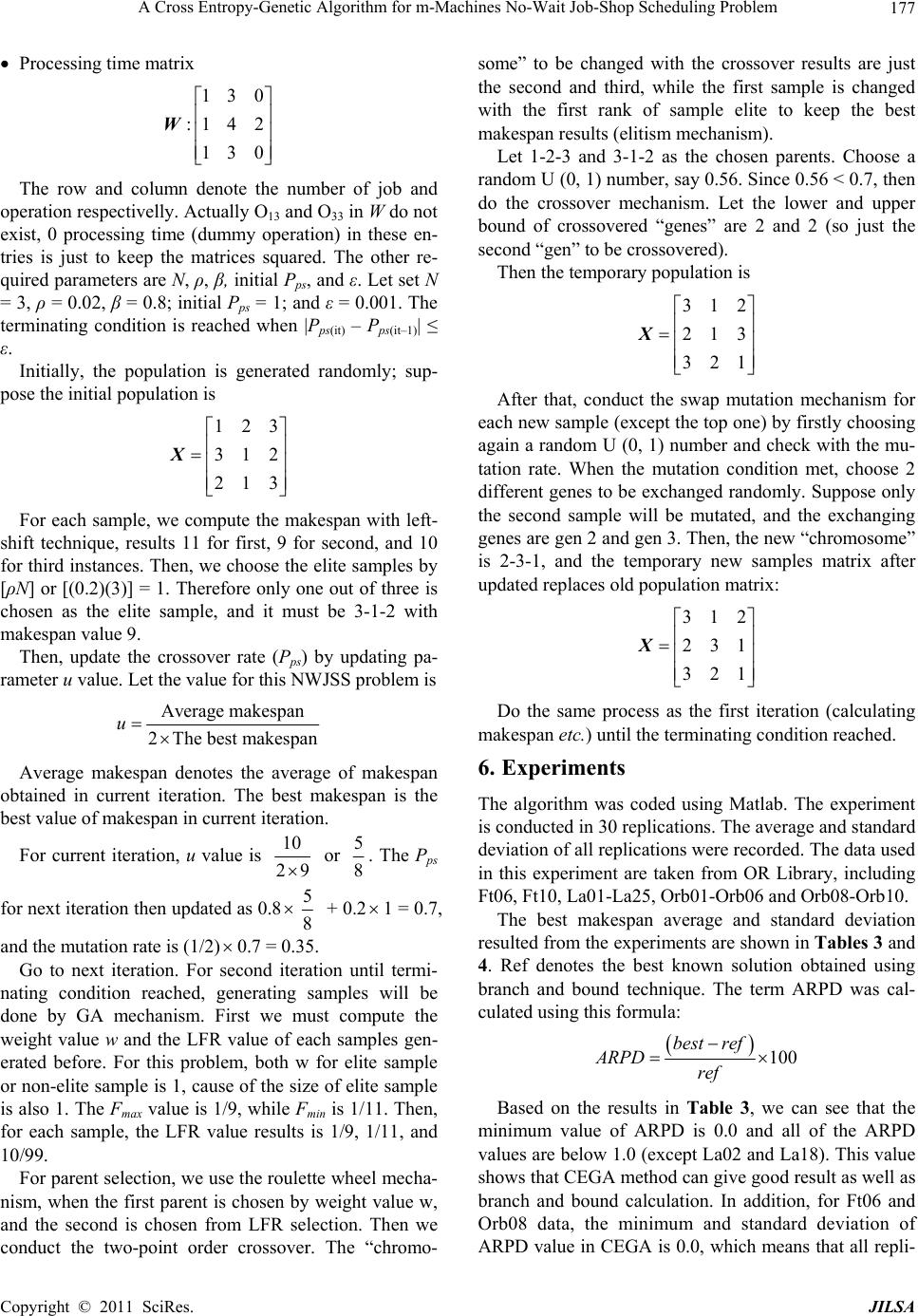

A Cross Entropy-Genetic Algorithm for m-Machines No-Wait Job-Shop Scheduling Problem177
 Processing time matrix
130
:1 42
130





W
The row and column denote the number of job and
operation respectivelly. Actually O13 and O33 in W do not
exist, 0 processing time (dummy operation) in these en-
tries is just to keep the matrices squared. The other re-
quired parameters are N, ρ, β, initial Pps, and ε. Let set N
= 3, ρ = 0.02, β = 0.8; initial Pps = 1; and ε = 0.001. The
terminating condition is reached when |Pps(it) – Pps(it–1)| ≤
ε.
Initially, the population is generated randomly; sup-
pose the initial population is
123
312
213





X
For each sample, we compute the makespan with left-
shift technique, results 11 for first, 9 for second, and 10
for third instances. Then, we choose the elite samples by
[ρN] or [(0.2)(3)] = 1. Therefore only one out of three is
chosen as the elite sample, and it must be 3-1-2 with
makespan value 9.
Then, update the crossover rate (Pps) by updating pa-
rameter u value. Let the value for this NWJSS problem is
Average makespan
2The best makespan
u
Average makespan denotes the average of makespan
obtained in current iteration. The best makespan is the
best value of makespan in current iteration.
For current iteration, u value is 10
29 or 5 8. The Pps
for next iteration then updated as 0.85
8 + 0.2

1 = 0.7,
and the mutation rate is (1/2)0.7 = 0.35.
Go to next iteration. For second iteration until termi-
nating condition reached, generating samples will be
done by GA mechanism. First we must compute the
weight value w and the LFR value of each samples gen-
erated before. For this problem, both w for elite sample
or non-elite sample is 1, cause of the size of elite sample
is also 1. The Fmax value is 1/9, while Fmin is 1/11. Then,
for each sample, the LFR value results is 1/9, 1/11, and
10/99.
For parent selection, we use the roulette wheel mecha-
nism, when the first parent is chosen by weight value w,
and the second is chosen from LFR selection. Then we
conduct the two-point order crossover. The “chromo-
some” to be changed with the crossover results are just
the second and third, while the first sample is changed
with the first rank of sample elite to keep the best
makespan results (elitism mechanism).
Let 1-2-3 and 3-1-2 as the chosen parents. Choose a
random U (0, 1) number, say 0.56. Since 0.56 < 0.7, then
do the crossover mechanism. Let the lower and upper
bound of crossovered “genes” are 2 and 2 (so just the
second “gen” to be crossovered).
Then the temporary population is
312
213
321











X
After that, conduct the swap mutation mechanism for
each new sample (except the top one) by firstly choosing
again a random U (0, 1) number and check with the mu-
tation rate. When the mutation condition met, choose 2
different genes to be exchanged randomly. Suppose only
the second sample will be mutated, and the exchanging
genes are gen 2 and gen 3. Then, the new “chromosome”
is 2-3-1, and the temporary new samples matrix after
updated replaces old population matrix:
312
231
321











X
Do the same process as the first iteration (calculating
makespan etc.) until the terminating condition reached.
6. Experiments
The algorithm was coded using Matlab. The experiment
is conducted in 30 replications. The average and standard
deviation of all replications were recorded. The data used
in this experiment are taken from OR Library, including
Ft06, Ft10, La01-La25, Orb01-Orb06 and Orb08-Orb10.
The best makespan average and standard deviation
resulted from the experiments are shown in Tables 3 and
4. Ref denotes the best known solution obtained using
branch and bound technique. The term ARPD was cal-
culated using this formula:


100
best ref
ARPD ref


Based on the results in Table 3, we can see that the
minimum value of ARPD is 0.0 and all of the ARPD
values are below 1.0 (except La02 and La18). This value
shows that CEGA method can give good result as well as
branch and bound calculation. In addition, for Ft06 and
Orb08 data, the minimum and standard deviation of
ARPD value in CEGA is 0.0, which means that all repli-

A Cross Entropy-Genetic Algorithm for m-Machines No-Wait Job-Shop Scheduling Problem 178
Table 3. Performance of CEGA for small instances.
Size Makespan CEGA Time (sec)
Instances Job/
Mach
Ref Best Avg StDev ARPD AvgStDev
ft06 6/6 73 73 73.0 0.0 0.0 7.10.1
la01 10/5 971 975 990.1 14.7 0.4 132.610.8
la02 10/5 937 961 970.9 9.0 2.5 141.16.1
la03 10/5 820 820 852.4 19.3 0.0 133.012.2
la04 10/5 887 887 891.7 8.8 0.0 130.112.7
la05 10/5 777 781 788.0 11.4 0.5 149.312.4
ft10 10/10 16071607 1611.9 12.4 0.0 269.412.1
orb01 10/10 16151615 1630.6 20.2 0.0 307.824.2
orb02 10/10 14851485 1509.2 14.8 0.0 240.410.8
orb03 10/10 15991599 1620.2 19.8 0.0 295.816.9
orb04 10/10 16531653 1692.7 39.3 0.0 278.514.0
orb05 10/10 13651370 1390.3 18.7 0.4 257.114.9
orb06 10/10 15551555 1559.1 15.5 0.0 284.215.0
orb08 10/10 13191319 1319.0 0.0 0.0 291.73.4
orb09 10/10 14451445 1482.6 39.2 0.0 270.723.2
orb10 10/10 15571557 1585.6 16.2 0.0 253.417.7
la16 10/10 15751575 1581.5 19.9 0.0 250.913.6
la17 10/10 13711384 1405.5 24.9 0.9 241.521.6
la18 10/10 14171507 1509.7 9.1 6.0 240.017.8
la19 10/10 14821491 1531.4 34.8 0.6 253.27.4
la20 10/10 15261526 1542.5 28.8 0.0 255.811.4
Table 4. Performance of CEGA for large instances.
Size Makespan CEGA Time (sec)
Instan
ces Job/
Mach
Ref Best Avgstd ARPD Avg std
la06 15/5 1248 1304 1342.024.3 4.3 1635.8236.9
la07 15/5 1172 1221 1265.723.9 4.0 1670.1205.8
la08 15/5 1244 1274 1323.823.2 2.4 1626.9187.2
la09 15/5 1358 1382 1443.121.2 1.7 1745.9202.6
la10 15/5 1287 1299 1353.930.7 0.9 1624.3250.6
la11 20/5 1671 1722 1793.531.9 3.0 10061.71097.2
la12 20/5 1452 1538 1597.926.2 5.6 9695.11102.8
la13 20/5 1624 1674 1759.130.7 3.0 10525.01028.4
la14 20/5 1691 1749 1821.431.6 3.3 9976.71199.6
la15 20/5 1694 1752 1851.941.3 3.3 10722.11237.0
la21 15/10 2048 2054 2209.862.1 0.3 3032.3426.2
la22 15/10 1887 1910 1972.142.1 1.2 2970.9418.5
la23 15/10 2032 2098 2184.045.2 3.1 2995.8429.7
la24 15/10 2015 2056 2133.636.9 2.0 2889.1332.4
la25 15/10 1917 1994 2059.431.7 3.9 3049.5458.7
cations gives the optimal value. Based on this result, we
can conclude that the performance of CEGA is relatively
well, especially for small instances.
For larger size problem, CEGA’s performance tends to
decline. Based on the result in Table 4, we can see that
most of the ARPD values are greater than 1.0. It is oc-
curred because the increase of jobs number processed
will increase the number of search space as factorial. For
example, when the job number increases from 10 to 15
jobs, the search space increases from 10! to 15! or 15 ×
14 × 13 × 12 × 11 = 360360 times larger than 10 jobs.
This increase, of course is hard to be followed by the
number of sample size. However, by using n3 number of
sample, we can say that this algorithm still has a good
tolerable performance. This is indicated by the ARPD
values which are less than 1.0 (for example in La10 and
La21) and most of ARPD value are still less than stan-
dard error 5.0 (except La12).
Based on the result shown by Tables 3 and 4, the best
and average makespan value obtained from all replica-
tions, tends to have a close value with the reference
makespan that shows that the t to the result 3 and Table
4, the algorithm’s performance is good enough. Mean-
while, the standard deviation tends to be large (greater
than 10.0, except in certain cases). This means that the
algorithm produces non-uniform makespan at each repe-
tition. But, the probability of getting best result is rela-
tively higher. To assure that the result not to converge to
a local optimum, this algorithm actually needs to be op-
timized again. By reducing the standard deviation value
with better or at least same average value (which means
the makespan values obtained at each repetition will be
more uniform but still tend to approach best value of
reference).
Although this algorithm produces better makespans,
the computation time is relatively long and will increase
significantly when the job size are getting larger. This
fact can be seen on Figure 2, where the average time
needed by this algorithm and standard deviation value
increase drastically as the job size increases. This is al-
leged to be caused by timetabling process to calculate the
objective function which is relatively time consuming.
As explained previously that simple shift timetabling
method used requires checking for the presence of over-
load on the machine for each new job scheduled. Every
will-be-scheduled-job has a specific machine overload
when it is being scheduled. It must be shifted as far as
the relevant value of time of overload on that machine.
After being moved, the other machines are overload.
Then the shifting must be done again until all of ma-
chines have no overload. This mechanism certainly takes
a long computing time, especially when the size of the
jobs is getting larger. The use of lower level program-
ming language such as C or C++ can improve computa-
tional time performance.
Compared with other algorithms, such as Genetic Al-
gorithm-Simulated Annealing [2] and Hybrid Tabu
Search [3], CEGA performance can be shown in Tables
5 and 6. Highlighted in bold is the best makespan for
each instance. Reference makespans (Ref), for small in-
stances, are the optimum value obtained by branch and
bound algorithm. For large instances are the best known
makespan ever obtained by researchers until present [8].
Based on the comparison in Table 5, for small in-
stances, we can see that the performance of CEGA is
absolutely better than GASA in terms of makespan. Out
of 21 instance, CEGA can reach 18 optimal makespan
values better than GASA which only reach only 4 in-
C opyright © 2011 SciRes. JILSA

A Cross Entropy-Genetic Algorithm for m-Machines No-Wait Job-Shop Scheduling Problem179
Table 5. Makespan comparison of GASA, HTS and CEGA
for small instances.
GASA HTS CEGA
Instance Ref Best ARPD Best ARPD Best ARPD
ft06 73 73 0.0 73 0.0 73 0.0
la01 971 1037 6.4 975 0.4 9750.4
la02 937 990 5.4 975 4.1 9612.5
la03 820 832 1.4 820 0.0 8200.0
la04 887 889 0.2 889 0.2 8870.0
la05 777 817 4.9 777 0.0 7810.5
ft10 1607 1620 0.8 1607 0.0 16070.0
orb01 1615 1663 2.9 1615 0.0 16150.0
orb02 1485 1555 4.5 1518 2.2 14850.0
orb03 1599 1603 0.2 1599 0.0 15990.0
orb04 1653 1653 0.0 1653 0.0 16530.0
orb05 1365 1415 3.5 1367 0.1 13700.4
orb06 1555 1555 0.0 1557 0.1 15550.0
orb08 1319 1319 0.0 1319 0.0 13190.0
orb09 1445 1535 5.9 1449 0.3 14450.0
orb10 1557 1618 3.8 1571 0.9 15570.0
la16 1575 1637 3.8 1575 0.0 15750.0
la17 1371 1430 4.1 1384 0.9 13840.9
la18 1417 1555 8.9 1417 0.0 15076.0
la19 1482 1610 8.0 1491 0.6 14910.6
la20 1526 1693 9.9 1526 0.0 15260.0
Average 3.5 0.52 0.5
Table 6. Makespan comparison of GASA, HTS and CEGA
for large instances.
GASA HTS CEGA In-
stances Ref Best ARPD Best ARPD BestARPD
la06 1248 1339 6.8 1248 0.0 13044.3
la07 1172 1240 5.5 1172 0.0 12214.0
la08 1244 1296 4.0 1298 4.2 12742.4
la09 1358 1447 6.2 1415 4.0 13821.7
la10 1287 1338 3.8 1345 4.3 12990.9
la11 1671 1825 8.4 1704 1.9 17223.0
la12 1452 1631 11.0 1500 3.2 15385.6
la13 1624 1766 8.0 1696 4.2 16743.0
la14 1691 1805 6.3 1722 1.8 17493.3
la15 1694 1829 7.4 1747 3.0 17523.3
la21 2048 2182 6.1 2191 6.5 20540.3
la22 1887 1965 4.0 1922 1.8 19101.2
la23 2032 2193 7.3 2126 4.4 20983.1
la24 2015 2150 6.3 2132 5.5 20562.0
la25 1917 2034 5.8 2020 5.1 19943.9
Average 6.5 3.3 2.8
stance. The average ARPD resulted by GASA is also
larger than the average ARPD resulted by CEGA. Com-
paring CEGA with HTS shows that CEGA is better than
HTS in terms of makespan. HTS reach 14 optimal
makespan which is less than those of CEGA. Though,
the ARPD of HTS is better than CEGA.
For larger instances, as shown in Table 6, compared to
GASA and HTS, generally CEGA performed better.
CEGA dominates 9 out of 15 instances, while the rest is
outperformed by HTS. For all those instances, all the
three methods; GASA, HTS and CEGA; can not reach
the ever best makespan values. In terms of ARPD, the
performance of CEGA is slightly better than HTS.
7. Conclusions
We have applied hybrid cross entropy-genetic algorithm
(CEGA) to solve NWJSS. We can conclude that CEGA
can be used as an alternative tool to solve NWJSS prob-
lem and can be applied widely on many industries with
NWJSS characteristics. For small instances CEGA per-
formed well in terms of makespan and computation time.
Generally, CEGA performance is better than the Genetic
Algorithm-Simulated Annealing (GASA) and Hybrid
Tabu Search (HTS), especially for small size instances.
In the future research, CEGA for NWJSS must be modi-
fied to get better performance especially for the large
size instances. The implementation using lower level
programming language might improve the performance
of CEGA. On the other hand, this algorithm application
on the other problems is also suggested.
8. References
[1] P. J. Chao-Hsien and H. Han-Chiang, “A Hybrid Genetic
Algorithm for No-Wait Job Shop Scheduling Problems,”
Expert Systems with Application, Vol. 36, No. 2, Part 2,
2009, pp. 5800-5806.
doi:10.1016/j.eswa.2008.07.005
[2] C. J. Schuster and J. M. Framinan, “Approximative Pro-
cedures for No-Wait Job Shop Scheduling,” Operations
Research Letters, Vol. 31, No. 4, 2003, pp. 308-318.
doi:10.1016/S0167-6377(03)00005-1
[3] W. Bożejko and M. Makuchowski, “A Fast Hybrid Tabu
Search Algorithm for the No-Wait Job Shop Problem,”
Computers & Industrial Engineering, Vol. 56, No. 4,
2009, pp. 1502-1509.
doi:10.1016/j.cie.2008.09.023
[4] R.Y. Rubinstein and D. P. Kroese, “The Cross-Entropy
Method: A Unified Approach to Combinatorial Optimi-
zation. Monte-Carlo Simulation and Machine Learning,”
Springer Verlag, New York, 2004.
[5] C. F. Liaw, “An efficient Simple Metaheuristic for Mini-
mizing the Makespan in Two-Machine No-Wait Job
Shops,” Computer & Operations Research, Vol. 35, No.
10, 2008, pp. 3276-3283.
doi:10.1016/j.cor.2007.02.017
[6] A. Mascis and D. Pacciarelli, “Discrete Optimization:
Job-Shop Scheduling with Blocking and No-Wait Con-
straints,” European Journal of Operational Research,
Vol. 143, No. 3, 2002, pp. 498-517.
doi:10.1016/j.cor.2007.02.017
[7] J. M. Framinan and C. J. Schuster, “An Enhanced Time-
tabling Procedure for the No-Wait Job Shop Problem: a
Complete Local Search with Memory Approach,” Com-
puters & Operations Research, Vol. 33, No. 1, 2006, pp.
1200-1213. doi:10.1016/j.cor.2004.09.009
[8] J. Zhu, X. Li and Q. Wang, “Complete Local Search with
Limited Memory Algorithm for No-Wait Job Shops to
Minimize Makespan,” European Journal of Operational
Research, Vol. 198, No. 2, 2009, pp. 378-386.
doi:10.1016/j.ejor.2008.09.015

A Cross Entropy-Genetic Algorithm for m-Machines No-Wait Job-Shop Scheduling Problem 180
[9] M. Derek, “A Sequential Scheduling Approach to Com-
bining Multiple Object Classifiers Using Cross-Entropy,”
In: T. Windeatt and F. Roli, Eds., MCS 2003, LNCS 2709,
Springer-Verlag, Berlin, pp. 135-145.
[10] D. P. Kroese and K. P. Hui, “Applications of the Cross-
Entropy Method in Reliability Computational Intelli-
gence,” Reliability Engineering (SCI), Vol. 40, 2007, pp.
37-82.
[11] B. Santosa and N. Hardiansyah, “Cross Entropy Method
for Solving Generalized Orienteering Problem,” iBusi-
ness, Vol. 2, No. 4, 2010, pp. 342-347.