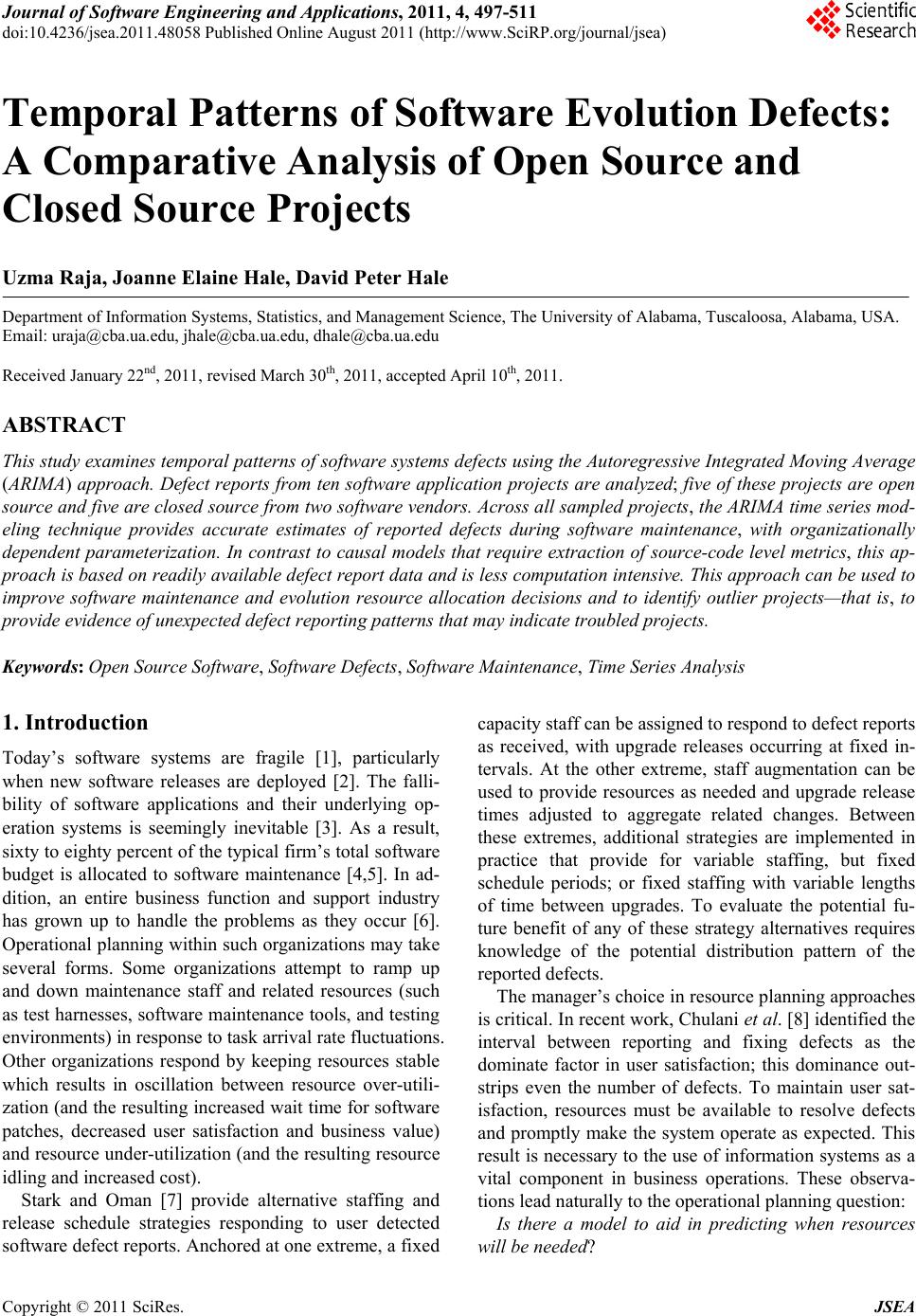
 Journal of Software Engineering and Applications, 2011, 4, 497-511 doi:10.4236/jsea.2011.48058 Published Online August 2011 (http://www.SciRP.org/journal/jsea) Copyright © 2011 SciRes. JSEA 497 Temporal Patterns of Software Evolution Defects: A Comparative Analysis of Open Source and Closed Source Projects Uzma Raja, Joanne Elaine Hale, David Peter Hale Department of Information Systems, Statistics, and Management Science, The University of Alabama, Tuscaloosa, Alabama, USA. Email: uraja@cba.ua.edu, jhale@cba.ua.edu, dhale@cba.ua.edu Received January 22nd, 2011, revised March 30th, 2011, accepted A pr i l 10 th, 2011. ABSTRACT This study examines temporal patterns of software systems defects using the Autoregressive Integrated Moving Average (ARIMA) approach. Defect reports from ten software application projects are analyzed; five of these projects are open source and five are closed source from two software vendors. Across all samp led projects, the ARIMA time series mod- eling technique provides accurate estimates of reported defects during software maintenance, with organizationally dependent parameterization. In contrast to causal models that require extraction of source-code level metrics, this ap- proach is based on readily available defect report data and is less computation intensive. This approach can be used to improve software maintenance and evolution resource allocation decisions and to identify outlier projects—that is, to provide evidence of unexpected defect reporting patterns that may indicate troubled projects. Keywords: Op en Source Software, Software Defects, Software Maintenance, Time Series Analysis 1. Introduction Today’s software systems are fragile [1], particularly when new software releases are deployed [2]. The falli- bility of software applications and their underlying op- eration systems is seemingly inevitable [3]. As a result, sixty to eighty percent of the typical firm’s total software budget is allocated to software maintenance [4,5]. In ad- dition, an entire business function and support industry has grown up to handle the problems as they occur [6]. Operational planning within such organizations may take several forms. Some organizations attempt to ramp up and down maintenance staff and related resources (such as test harnesses, software maintenance tools, and testing environments) in response to task arrival rate fluctuations. Other organizations respond by keeping resources stable which results in oscillation between resource over-utili- zation (and the resulting increased wait time for software patches, decreased user satisfaction and business value) and resource under-utilizatio n (and the resulting resource idling and increased cost). Stark and Oman [7] provide alternative staffing and release schedule strategies responding to user detected software defect reports. Anchored at one extreme, a fixed capacity staff can be assigned to respond to defect re ports as received, with upgrade releases occurring at fixed in- tervals. At the other extreme, staff augmentation can be used to provide resources as needed and upgrade release times adjusted to aggregate related changes. Between these extremes, additional strategies are implemented in practice that provide for variable staffing, but fixed schedule periods; or fixed staffing with variable lengths of time between upgrades. To evaluate the potential fu- ture benefit of any of these strategy alternatives requires knowledge of the potential distribution pattern of the reported defe cts. The manager’s choice in resource planning approaches is critical. In recent work, Chulani et al. [8] identified the interval between reporting and fixing defects as the dominate factor in user satisfaction; this dominance out- strips even the number of defects. To maintain user sat- isfaction, resources must be available to resolve defects and promptly make the system operate as expected. This result is necessary to the use of information systems as a vital component in business operations. These observa- tions lead naturally to the operational planning question: Is there a model to aid in predicting when resources will be needed?  Temporal Patterns of Software Evolution Defects: A Comparative Analysis of Open Source and Closed Source Projects 498 Secondarily, if such a predictive model for software maintenance resources can be derived: Is such a predictive model computationally and eco- nomically practi cal? These questions have yet to be adequately addressed, as according to Pelayo and Dick [9] “no parametric model has ever been developed that accurately forecasts the number or occurrence of faults [defects] in a software module.” To meet this research challenge, this study seeks to develop an accurate predictive model of soft- ware defect patterns that can be applied to the larger problem of software maintenance resource allocation and alignment, while using readily available defect report data and computational resources. 2. Background During peak shopping times, retailers increase their staff of floor professionals and cashiers. When few truckloads are expected to arrive, a distribution center manager schedules fewer fork lift operators. Software mainte- nance managers are faced with similar arrival rate fluc- tuations that impact resource requirements. Software maintenance managers must ensure product quality and required service levels, while simultaneously minimizing costs associated with defect resolution and penalties for non-performance [10,11]. Faced with this challenge, formal predictive models are not common in resource planning; instead maintenance planning methods in prac- tice continue to be largely ad hoc [12], with recent per- sonal experience weighing heavily on practitioner pre- dictions of change requests and staffing needs [10,12]. As a result, maintenance project managers too often ei- ther overstaff (causing resources to idle and costs to in- crease) or understaff (causing delays in defect resolution and a decline in user satisfaction and business value). Previous work is reviewed regarding predicting soft- ware defects, where a defect is defined as a reported error that is encountered in an operational software applicatio n. The predominance of prior research does not focus on patterns of discovered defects once the application is in use. Instead, a strong body of research exists that predicts software defects during the development of new systems. Both areas are explored and fall into three classes of forecasting approaches: causal, learning and time-series. 2.1. Causal Models Many researchers have constructed models to predict the number of defects remaining in completed software products or identify defect-dense modules within a sys- tem. Ohlsson et al. [13] use principal components analy- sis and classification trees to identify fault-prone com- ponents. Khoshgoftaar and Lanning [14] used a neural network technique to classify modules as high or low risk for defects based on quality and complexity metrics in- cluding the number of fault-correcting and enhancive changes. El Emam and Laitenberger [15] used a Monte Carlo simulation to evaluate the accuracy of a capture- recapture re-inspection de fe c t prediction model. Khoshgoftaar et al. [16] constructed a nonlinear re- gression model predicting the number of faults using lines of code. Fenton and Neil [17] and Adams [18] dis- covered that post-release defects were more likely in modules where few defects were discovered pre-release and that testing effectiveness significantly impacts the post-release presence of defects. Krishnan and Kellner [19] found that organizations that consistently followed Capability Maturity Mo del (CMM) practices ex perienced significantly fewer reported field defects in the resulting software. Krishnan [20] found that higher levels of do- main experience of the software team are associated with a reduction in the number of field defects in the product. However, there is no significant association between either the language or the domain experience of the software team and the costs incurred in developing the product. Such causal predictive models of defects identify the factors that impact software defects, thus serving both predictive and explanatory roles regarding what factors could be controlled to manage future defects. Such mod- els are useful for software development teams, since they can control these variables and manage the overall qual- ity of software system. Most of these models however require access to internal characteristics of software. Although available for decades for use in staffing and system quality and defect modeling, these causal models have not been widely used in practice because of the cost and complexity of implementation [21]. Further compli- cating their use during software maintenance, mainte- nance practitioners have little control over the internal characteristics commonly modeled to predict defects (largely set at time of product release), thus rendering such complex models of little use to maintenance man- agers who want to manage and allocate budget, time and resources for future defect occurrences. 2.2. Learning Techniques A number of authors have investigated the use of ma- chine-learning techniques for software defect prediction. Some examples include neural networks [22], genetic programming [23], fuzzy clustering ([24] and decision trees [25]. For example, Seliya et al. [26] proposed a semi-supervised clustering method to detect failures in software modules. Instead of working with the individual modules on software, they group modules and label them as fault prone or not fault prone. Fenton and Neil [17] used Bayesian belief networks (BBN) as an effective approach for defect prediction, an Copyright © 2011 SciRes. JSEA  Temporal Patterns of Software Evolution Defects: A Comparative Analysis of Open Source and Closed Source Projects499 ptpt approach that is gaining popular ity [27]. Building on this work, Menzies et al. [28] showed positive results using a naïve Bayes classifier with log-filtered static code meas- ures. Challagulla et al. [29] used simulation to compare software prediction using stepwise regression, rule in- duction, case-based reasoning, and artificial neural net- works. They concluded that stepwise regression per- formed better with contin uous target functions, while the other machine learning approaches performed better for discontinuous target functions. They favored case based reasoning since it appeared to be the best all round pre- dictor by a small margin. Song et al. [30] investigated the above prediction models on real software data, compar- ing them in terms of accuracy, explanatory value, and configurability. They concluded that the explanatory value of case-based reasoning and rule induction gives them an advantage over neural nets, which have prob- lems of configuration. Aljahdali et al. [31] compared regression with neural nets for prediction of software reliability and concluded that for most cases neural nets provided fewer errors than regression models. These adaptive, learning based predictive models have been found to i mprove on the accuracy of traditional sta- tistical linear causal models. However, they still fail to meet the ease of implementation goal of this study, as they require professionals with specialized model know- ledge and sophisticated software not typically at the dis- posal of a maintenance manager. 2.3. Time Series Models Causal and learning models are both computationally complex and require significant investments in project data collection. In response to these challenges, the goal of this study is to provide a method of predicting patterns in software defects that is accurate without the cost and complexity of more traditional predictive methods. Time series models assume that events are correlated over time and the impact of other factors is progressively captured in historical archives [32]. The most commonly used forecasting method, time series models are fre- quently used to predict product demand [33], macro-eco- nomic trends [34], and retail sales [35], but are yet to be widely adopted in the software maintenance domain [36]. Within the domain of software maintenance, time se- ries modeling has had limited use. Kemerer and Slaugh- ter [37] used ARIMA modeling to predict monthly changes, not reported defects, in software. Kenmei et al. [38] and Raja et al. [36] created time series models for defects in open source software (OSS) and found that the ARIMA models outperform the accuracy of simple mod- els. Each research team found that time series modeling was a suitable and accurate method of defect prediction for large-scale OSS projects. However neither of the lat- ter studies investigated proprietary closed source soft- ware applications. Thus based on results in the literature, time series analysis potentially provides a method of predicting pat- terns in software defects that is accurate without the cost and complexity of causal and learning models. It is left to this study to determine whether the results found in OSS projects can be replicated across open and closed source software (CSS) applications. 3. Methods This work builds on previous studies that discovered the accuracy and ease of implementation of time series soft- ware defect prediction. Specifically this research com- pares the defect evolution patterns across a diverse set of projects, providing the opportunity to study projects within and across organizations. This section describes the prediction model adopted in this study, the software maintenance projects examined, the associated data ex- tracted, and the analytical techniques used. 3.1. Time Series Analysis As proposed in prior studies [32,36], time series an alysis offers promise in the field of software defect prediction. These models are suited for representing situations char- acterized by frequent variations, such as the pattern of software defect occurrences. A time series is a collection of observations made over equal intervals of time that can be used to predict future values and to identify trends [39] . A wide variety of time series modeling techniques are available and their su itability depends upon the nature of the data. A Moving Average series (MA) explain present as a mixture of random impulses, while an Autoregres- sive (AR) model builds the present in terms of past val- ues. These series are suitable for data that is stationary in nature i.e. its statistical properties (e.g. mean, variance, autocorrelation) are constant over time. For cases in which there is evidence of data being non-stationary as opposed to stationary, Box and Jenkins [40] introduced a corresponding generalized model. This model is called Autoregressive Integrated Moving Aver- age (ARIMA). T he general form of ARI M A (p,d,q) is: 011 11 t tqtq YYY (1) where: Yt = time series of the variable y. t = coefficient associated with Yt, to be estimated using least squares. t = the defect term, assumed to be independent, identically distributed variables sampled from a normal Copyright © 2011 SciRes. JSEA  Temporal Patterns of Software Evolution Defects: A Comparative Analysis of Open Source and Closed Source Projects 500 distribution with zero mean. t = the coefficient associated with t to be esti- mated using least squares. As detailed in the following subsections, the ARIMA modeling strategy followed in this study is comprised of four steps: Identification, Estimation, Diagnostic Testing and Application . Model Identification: The first step in model identifi- cation is often to apply a logarithmic transformation to stabilize the variance of a series. Then the model is pa- rameterized as ARIMA (p,d,q), where p = order of the Autoregressive component. d = order of the Dif ferenced com ponent. q = order of the Moving Average component. During model identification, the time series is ana- lyzed to assess what values of the parameters p, d, and q are most appropriate. The value of d is set taking into account whether the series is stationary (d = 0) or non- stationary (d > 0). Estimation: The original or transformed time series is then modeled using the parameters and identified in the previous step to estimate the coefficients in Equation (1). The different candidate values of p and q are used to compute the respective coefficient. The final model is selected using goodness of fit tests. Where goodness of fit is equivalent, t he m ost parsim onious m odel i s selected. Diagnostic Testing: The residuals are computed as the difference of the actual and predicted values (using the identified mode). These residuals are then analyzed using known techniques to determine the adequacy of the model. The residuals of a good model are expected to be small and random. Model Application: The predictive model accuracy on unseen data is estimated using a hold-out data sample [41]. Using this approach, a subset of the time series data is withheld from use in parameter estimation, and is in- stead used to test the model’s accuracy. 3.2. Site Selection and Data Description To study patterns in defect arrival rates, projects from a diverse set of organizations, problem domains, teams, and development methodologies were selected. The closed source software data was acquired from two or- ganizations. Organization A is a large diversified interna- tional software consulting firm, with a mature method- ology environment; all Organization A development groups are currently assessed at Capability Maturity Model Integration (CMMI) Level 3 or higher. Data for three Organization A projects was obtained, denoted in this study as Project A1, Project A2, and Project A3. Organization B is a small (30 employee) privately owned provider of financial transaction automation soft- ware using agile methodologies. Data for two Organiza- tion B projects was obtained, denoted in this study as Project B1 and Project B2. In addition to the five CSS projects (three from Or- ganization A and two from Organization B) five projects not included in Raja et al. [36] study were randomly se- lected from the list of the top twenty most active OSS projects within the SourceForge repository. Inclusion of these five projects provides process replication and ex- tends the sample set coverage by more than 50% to the OSS projects as evaluated by Raja et al. [36]. Descrip- tions of the OSS and CSS projects included in this study are presented in Table 1. Each of the ten studied projects has one or more arti- fact repositories that store information regarding various artifact types e.g. defects, patches, and feature requests. Defects of an individual project can be extracted using the unique defect repository identifier, available in each artifact. The defect data also includes the time of defect submission. The data is then aggregated to compute monthly defects for each project. Table 1 shows the st art date, number of months of available data and the total number of defects for each of the sampled projects. 3.3. Variable Specification and Data Extraction Time series modeling requires that data are gathered across equally spaced time intervals. Consistent with the commonly used resource planning interval, a monthly count of software defects was computed for each project. The model accuracy is sensitive to the length of historical data available. Therefore projects with a minimum 50 months of data available were used in the analysis. This also ensures that there is enough data available for hold- out sampling and testing of the accuracy of the model forecasts. For OSS projects, the SourceForge.net defect-tracking repository holds archives of defect reports for the pro- jects hosted by that community. Organization A and B host their own internal defect tracking repositories for trouble resolution. In all three environments, the data dictionary of the repository was used to identify the arti- fact repository of defects. SQL queries were used to ex- tract individual project defect data from the hosting ar- chive warehouse. Further queries were used to compute monthly statistics of the defects for each project indi- vidually. The monthly counts of defects were computed using the time stamps of each defect report. The resulting dataset contained the monthly defects for all OSS and CSS projects. 4. Analysis and Results 4.1. Model Identification The first step in model identification is to stabilize the Copyright © 2011 SciRes. JSEA  Temporal Patterns of Software Evolution Defects: A Comparative Analysis of Open Source and Closed Source Projects Copyright © 2011 SciRes. JSEA 501 Table 1. Sample description. Projects Description Months Total Defects wxWidgets wxWidgetsis a free C++ framework that facilitates cross platform soft- ware development, including GUIs, threads, sockets, database, file system access, etc 90 4843 Firewall Builder Object Oriented GUI and set of compliers for various firewall platform. Currently implemented compilers for iptables, ipfiler, OpenBSD, ipfw, Cisco PIC firewall routers access lists 93 1067 Netatalk Netatalk is a freely-available Open Source AFP fileserver. It also provides a kernel level implementation of the AppleTalk Protocol Suite. A *NIX/*BSD system running Netatalk is capable of serving many Macin- tosh clients simultaneously as an AppleShare file server (AFP), Apple- Talk router, *NIX/*BSD print server, and for accessing AppleTalk print- ers. 69 347 PhpWiki PhpWiki is a WikiWikiWeb clone in PHP. A WikiWikiWeb is a site where anyone can edit the pages through an HTML form. Multiple stor- age backends, dynamic hyperlinking, themeable, scriptable by plugins, full authentication, ACL's. 99 627 Open Source Projects Exult Exuit is a game engine for running Ultima7 on modern operating systems, plus a map editor and other tools for creating your own mods and games. 102 1675 Org A#1 A1 is an n-tier web-enabled wholesale billing application using J2EE and interfacing with an Oracle database. 58 3539 Org A#2 A2 is an object oriented service rating, pricing and discounting applica- tion using J2EE and interfacing with Oracle database. 60 1214 Org A#3 A3 is a performance management system providing KPI dashboards and analytics for monitoring and forecasting, built using a SOA and interfac- ing with most industry stan dard databases. 58 377 Org B#1 B1 is a payment processing application built on Microsoft platform that includes check scanning, image and data archival, courtesy amount rec- ognition and legal amount r ec og ni t io n. 54 1842 Closed Source Projects Org B#2 B2 is a merchant capture application that allows for the remote digital capture of check and payment data at the point of presentment and the bundled transmission for depo s i t i n to multiple accounts 54 582 means and variances by applying a logarithmic transfor- mation to the time series data. The next step is to plot: the autocorrelation factors (ACF), the correlation, at spe- cific lags, between the residuals of the data; and the par- tial autocorrelation factors (PACF). For each studied project the values of p (the autoregressive component) and q (the moving average component) are determined by examining the trends in the ACF and PACF plots. If ACF plots die out (i.e., disappear gradually) and PACF plots cut-off (i.e., disappear abruptly), this suggests that an autoregressive model is suitable (p > 0, q = 0). If the opposite is true, i.e. the ACF plots cut-off and PACF plots die-out, a Moving Average model is suitable (p = 0, q > 0). If both ACF and PACF die out, then the most appropriate model contains both a p and q parameter (i.e. a mixed model is called for). The ACF and the PACF plots are shown in Figures 1-3. The differencing term is obtained by examining if the series is stationary or not. In most software evolution studies, a simple differencing (i.e., d = 1), transforms the data to a near-linear series [42]. 4.2. Model Estimation For all five of the studied OSS projects the best fitting model was ARIMA (0,1,1). Though the OSS project set used in this study did not overlap with the project set used by Raja et al., [36] the best fitting model is consis- tent with their findings. It can be seen that for each OSS project the p value of the t-statistic is significant for MA1. The plots of the residual ACF and PACF indicate that the model provides suitable fit and there are no significant correlations in the residuals. The final estimates of the model parameter are shown in Table 2 and the ACF and PACF plots of the residuals are shown in Figure 4. The best model for all the three projects in Organiza- tion A was ARIMA (2,1,0). Several competing models were evaluated, but based on fit statistics and the residual analysis the same autoregressive model was the best fit for all three projects. The final estimates of the model pa- rameters for each of the sampled Organization A projects 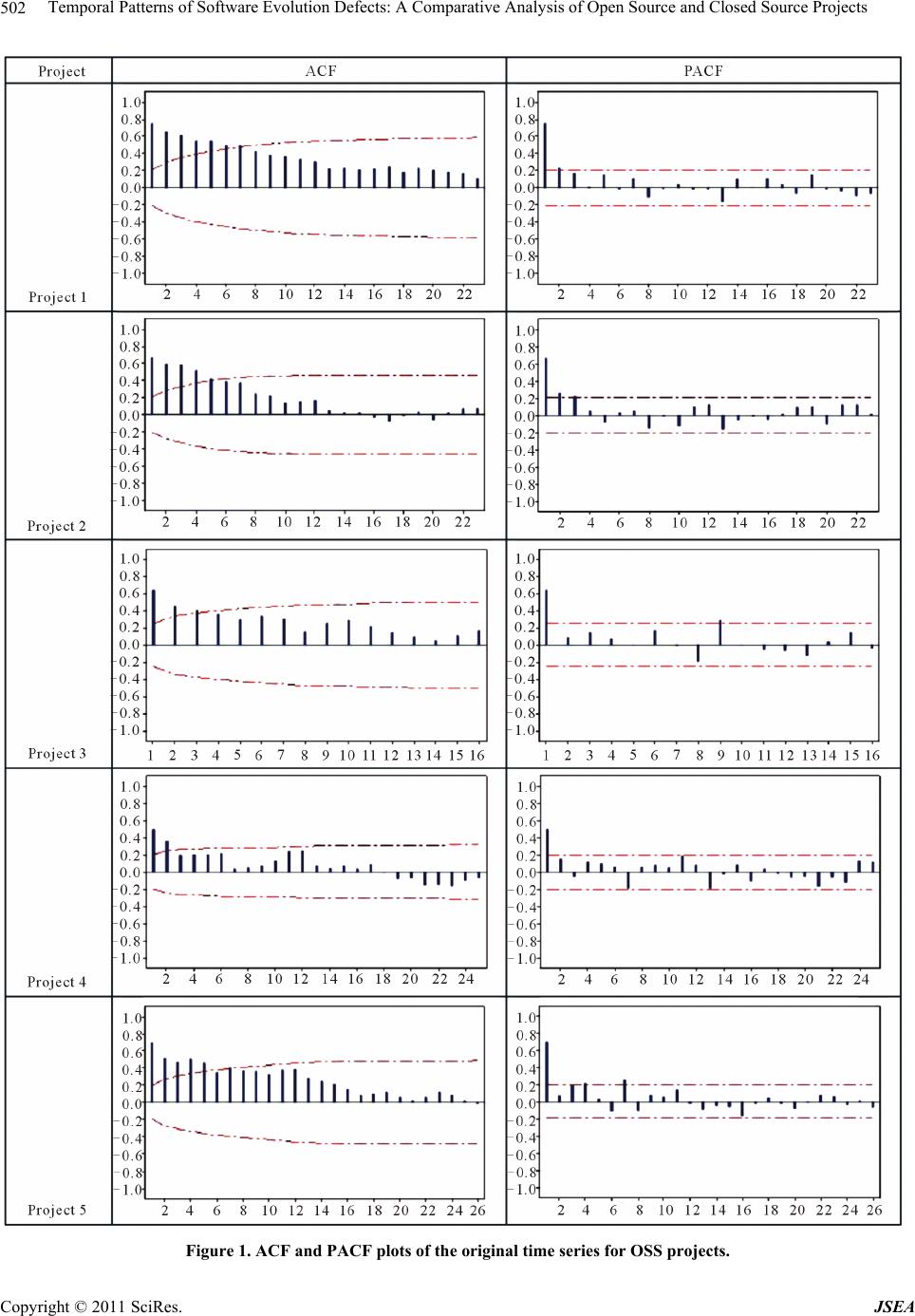 Temporal Patterns of Software Evolution Defects: A Comparative Analysis of Open Source and Closed Source Projects 502 Figure 1. ACF and PACF plots of the original time series for OSS projects. Copyright © 2011 SciRes. JSEA 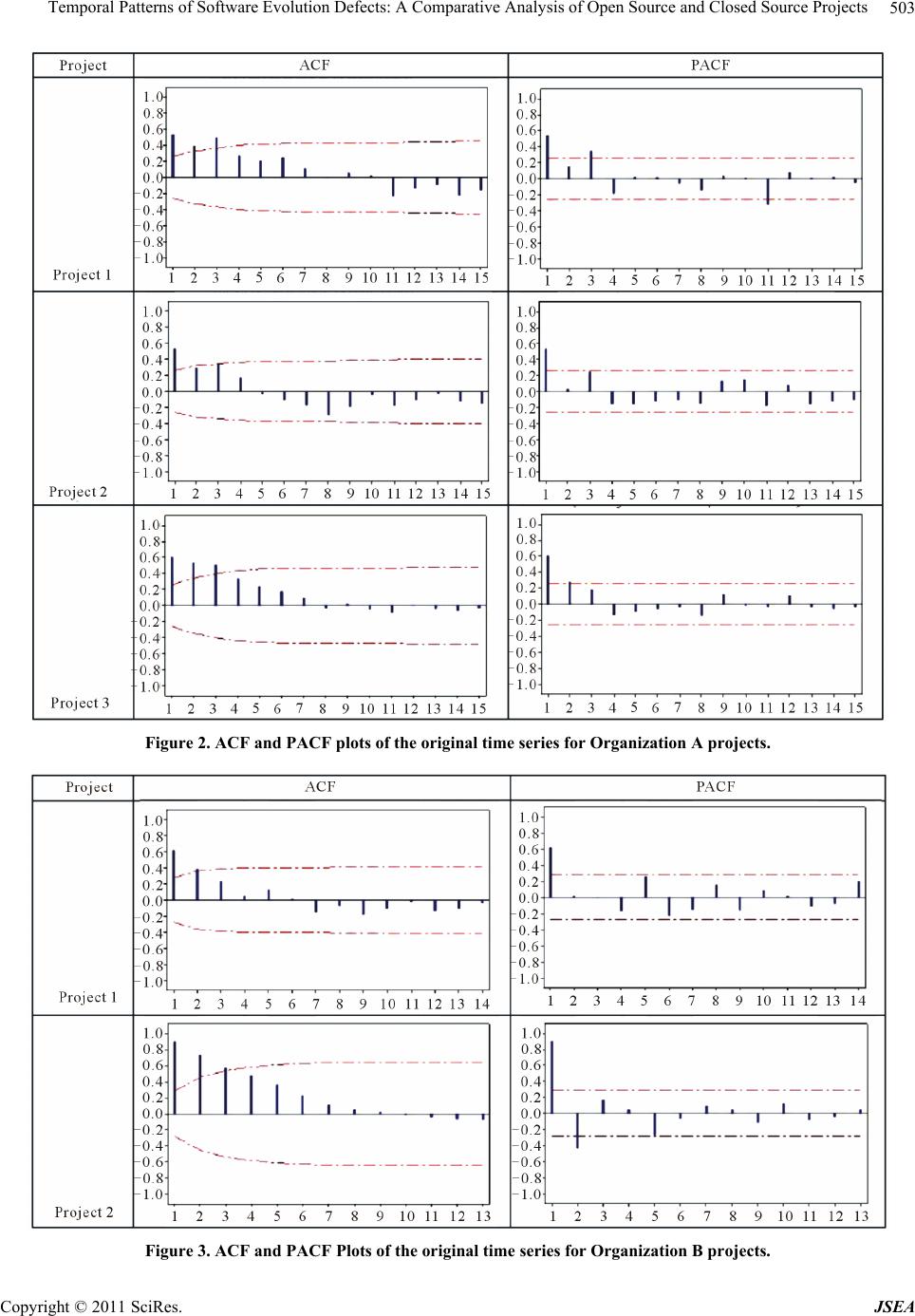 Temporal Patterns of Software Evolution Defects: A Comparative Analysis of Open Source and Closed Source Projects503 Figure 2. ACF and PACF plots of the original time series for Organization A projects. Figure 3. ACF and PACF Plots of the original time series for Organization B projects. Copyright © 2011 SciRes. JSEA  Temporal Patterns of Software Evolution Defects: A Comparative Analysis of Open Source and Closed Source Projects Copyright © 2011 SciRes. JSEA 504 Table 2. Best fitting model specifications for each project. Project Type Coefficient SE Coefficient t p OSS #1 MA1 Constant 0.5761 0.17 0.0873 0.6827 6.6 0.25 0 0.804 OSS #2 MA1 Constant 0.5606 –0.1085 0.0872 0.3075 6.43 –0.35 0 0.725 OSS #3 MA1 Constant 0.5693 –0.0854 0.1072 0.178 5.31 –0.48 0 0.633 OSS #4 MA1 Constant 0.6991 0.0005 0.0734 0.0242 9.53 0.02 0 0.984 OSS #5 MA1 Constant 0.6827 –0.0138 0.0743 0.0266 9.19 –0.52 0 0.604 Org A #1 AR1 AR2 Constant –0.5665 –0.5013 1.219 0.1245 0.1338 3.759 –4.55 –3.75 0.32 0 0 0.747 Org A #2 AR1 AR2 Constant –0.3478 –0.4101 0.376 0.1263 0.1275 1.74 –2.76 –3.25 0.22 0.008 0.002 0.83 Org A #3 AR1 AR2 Constant –0.8854 –0.6345 0.602 0.1089 0.1089 1.89 –8.13 –5.83 0.32 0 0 0.751 Org B #1 MA1 Constant 0.4163 –0.05461 0.128 0.05364 3.25 –1.02 0.002 0.313 Org B #2 MA1 Constant 0.3088 0.02648 0.151 0.07185 2.05 0.37 0.046 0.714 are shown in Table 2. The ACF and PACF plots of the residuals are shown in Figure 5. t model for both of the projects from Organization B was an ARIMA (0,1,1). Several competing models were evaluated, but based on fit statistics and the residual analysis the same Moving Average model was the best fit for both the projects. The final specifications of the model parameters for each of the sampled Organization B projects are shown in Table 2 and the ACF and PACF plots for Organization B are shown in Figure 6. 4.3. Diagnostic Testing After estimating the series for all the sample projects, they are individually tested ag ainst the competing models. The best model is selected using the t statistics and goodness of fit tests. The residuals are also analyzed to ensure that autocorrelation has been removed. We used the Ljung-Box [43] test for the residual analysis. The null hypothesis for this test is that ACFs for lag 1 through m are all 0. If H0 is rejected, it implies that there is signifi- cant autocorrelation in the residuals. Failure to reject the null hypothesis means that the co rrelation in the residuals is insignificant. The results of the diagno stic testing for all the projects are shown in Table 3. Across all 10 projects, diagnostic results show that the selected model fully captures the behavior of the series and there are no significant missing elements in the model. 4.4. Model Application Because the ultimate goal of the research is to develop models that can be useful for forecasting future defects, the accuracy of model predictions on unseen data is a critical factor. We therefore used the hold-out cross- validation technique for comparing model predictions [41]. In this method, some data is withheld and not used during parameter estimation. The selected model is then used to generate a forecast, which is compared to the withheld (ac t u a l ) values. We used a holdout sample of 4 months data for each project. This number was selected keeping in view the amount of data available for all projects. Results indicate the best-fit models identified in the Model Estimation section were all stable over the sample sets’ holdout se- ries for each of the 10 studied projects. Across all 10 sampled projects, the mean square error (MSE), mean absolute percentage error (MAPE), and mean absolute deviation (MAD) for the previously identified best-fit models (ARIMA (0,1,1) for OSS and Organization B; ARIMA (2,1,0) for Organization A) are all lower than competing models. 5. Discussions The purpose of this study is o determine whether a time t 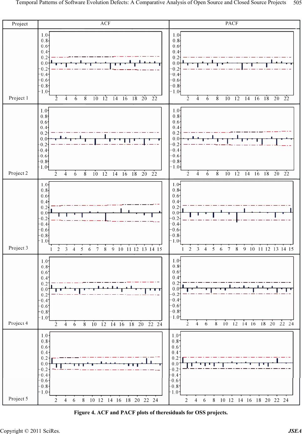 Temporal Patterns of Software Evolution Defects: A Comparative Analysis of Open Source and Closed Source Projects505 Figure 4. ACF and PACF plots of theresiduals for OSS pr ojec ts. Copyright © 2011 SciRes. JSEA 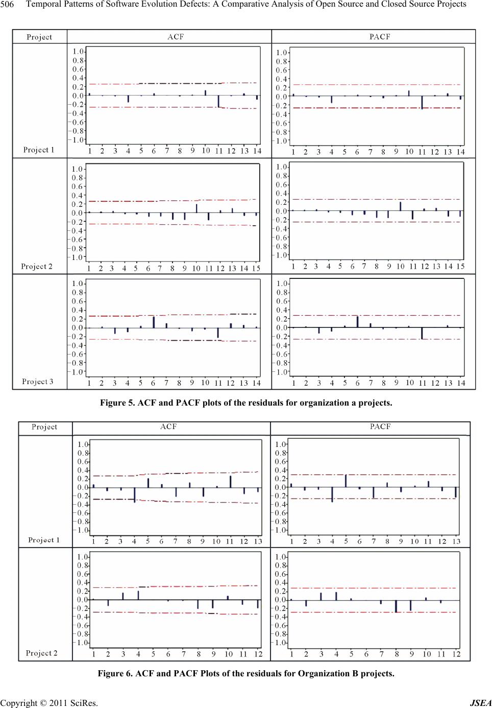 Temporal Patterns of Software Evolution Defects: A Comparative Analysis of Open Source and Closed Source Projects 506 Figure 5. ACF and PACF plots of the residuals for organization a projects. Figure 6. ACF and PACF Plots of the residuals for Organization B projects. Copyright © 2011 SciRes. JSEA 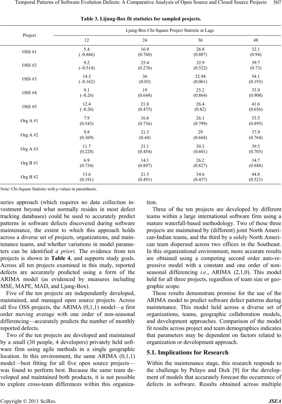 Temporal Patterns of Software Evolution Defects: A Comparative Analysis of Open Source and Closed Source Projects Copyright © 2011 SciRes. JSEA 507 Table 3. Lijung-Box fit statistics for sampled projects. Ljung-Box Chi-Square Project Statistic at Lags Project 12 24 36 48 OSS #1 5.4 (–0.866) 16.9 (0.768) 26.8 (0.807) 32.1 (0.94) OSS #2 9.2 (–0.514) 25.4 (0.276) 32.9 (0.522) 39.7 (0.73) OSS #3 14.3 (–0.162) 36 (0.03) 32.94 (0.061) 54.1 (0.193) OSS #4 9.1 (–0.26) 19 (0.648) 25.2 (0.864) 33.9 (0.908) OSS #5 12.4 (–0.26) 21.8 (0.475) 26.4 (0.82) 41.6 (0.656) Org A #1 7.9 (0.545) 16.6 (0.736) 26.1 (0.799) 33.5 (0.895) Org A #2 9.8 (0.369) 21.3 (0.44) 29 (0.668) 37.9 (0.764) Org A #3 11.7 (0.228) 21.1 (0.454) 30.3 (0.601) 39.5 (0.703) Org B #1 6.9 (0.734) 14.1 (0.897) 26.2 (0.827) 34.7 (0.888) Org B #2 13.6 (0.191) 21.5 (0.491) 34.6 (0.437) 44.8 (0.521) Note: Chi-Square Statistic with p values in parenthesis. series approach (which requires no data collection in- vestment beyond what normally resides in most defect tracking databases) could be used to accurately predict patterns in software defects discovered during software maintenance, the extent to which this approach holds across a diverse set of projects, organizations, and main- tenance teams, and whether variations in model parame- ters can be identified a priori. The evidence from ten projects is shown in Table 4, and supports study goals. Across all ten projects examined in this study, reported defects are accurately predicted using a form of the ARIMA model (as evidenced by measures including MSE, MAPE, MAD, and Ljung-Box). Five of the ten projects are independently developed, maintained, and managed open source projects. Across all five OSS projects, the ARIMA (0,1,1) model—a first order moving average with one order of non-seasonal differencing—accurately predicts the number of monthly reported defe cts. Two of the ten projects are developed and maintained by a small (30 people, 4 developers) privately held soft- ware firm using agile methods in a single geographic location. In this environment, the same ARIMA (0,1,1) model—best fitting for all five open source projects— was found to perform best. Because the same team de- veloped and maintained both products, it is not possible to explore cross-team differences within this organiza- tion. Three of the ten projects are developed by different teams within a large international software firm using a mature waterfall-based methodology. Two of these three projects are maintained by (different) joint North Ameri- can-Indian teams, and the third by a solely North Ameri- can team dispersed across two offices in the Southeast. In this organizational environment, more accurate results are obtained using a competing second order auto-re- gressive model with a constant and one order of non- seasonal differencing i.e., ARIMA (2,1,0). This model held for all three projects, regardless of team size or geo- graphic scope. These results demonstrate promise for the use of the ARIMA model to predict software defect patterns during maintenance. This model held across a diverse set of organizations, teams, geographic collaboration models, and development approaches. Comparison of the model fit results across project and team demographics indicates that parameters may be dependent on factors related to organization or development approach. 5.1. Implications for Research Within the maintenance stage, this research responds to the challenge by Pelayo and Dick [9] for the develop- ment of models that accurately forecast the occurrence of defects in software. Results obtained across multiple 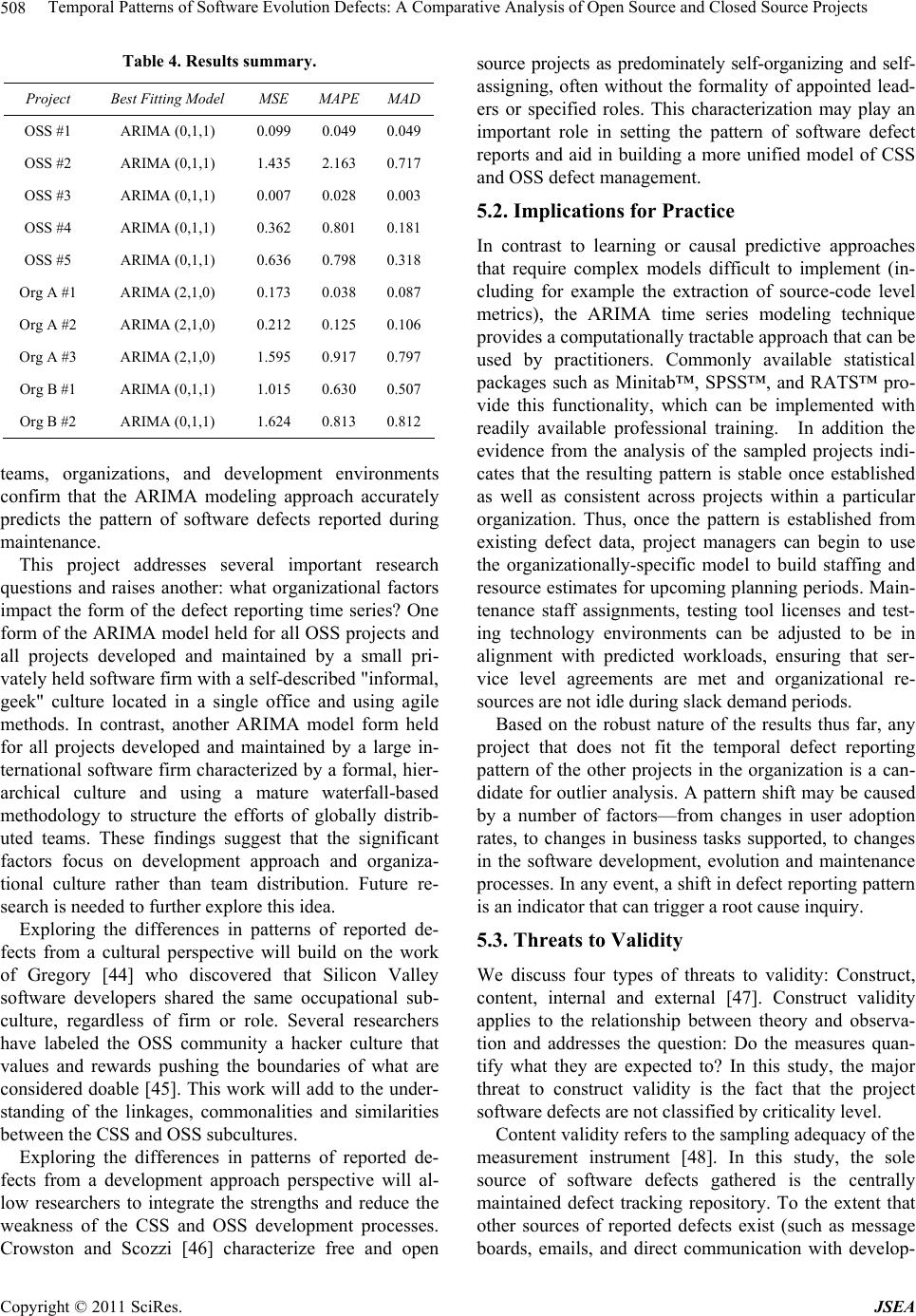 Temporal Patterns of Software Evolution Defects: A Comparative Analysis of Open Source and Closed Source Projects 508 Table 4. Results summary. Project Best Fitting Model MSE MAPE MAD OSS #1 ARIMA (0,1,1) 0.099 0.049 0.049 OSS #2 ARIMA (0,1,1) 1.435 2.163 0.717 OSS #3 ARIMA (0,1,1) 0.007 0.028 0.003 OSS #4 ARIMA (0,1,1) 0.362 0.801 0.181 OSS #5 ARIMA (0,1,1) 0.636 0.798 0.318 Org A #1 ARIMA (2,1,0) 0.173 0.038 0.087 Org A #2 ARIMA (2,1,0) 0.212 0.125 0.106 Org A #3 ARIMA (2,1,0) 1.595 0.917 0.797 Org B #1 ARIMA (0,1,1) 1.015 0.630 0.507 Org B #2 ARIMA (0,1,1) 1.624 0.813 0.812 teams, organizations, and development environments confirm that the ARIMA modeling approach accurately predicts the pattern of software defects reported during maintenance. This project addresses several important research questions and raises another: what organizational factors impact the form of the defect reporting time series? One form of the ARIMA model held for all OSS projects and all projects developed and maintained by a small pri- vately held software firm with a self-described "informal, geek" culture located in a single office and using agile methods. In contrast, another ARIMA model form held for all projects developed and maintained by a large in- ternational software firm characterized by a formal, hier- archical culture and using a mature waterfall-based methodology to structure the efforts of globally distrib- uted teams. These findings suggest that the significant factors focus on development approach and organiza- tional culture rather than team distribution. Future re- search is needed to further explore this idea. Exploring the differences in patterns of reported de- fects from a cultural perspective will build on the work of Gregory [44] who discovered that Silicon Valley software developers shared the same occupational sub- culture, regardless of firm or role. Several researchers have labeled the OSS community a hacker culture that values and rewards pushing the boundaries of what are considered doable [45]. This work will add to the under- standing of the linkages, commonalities and similarities between the CSS and OSS subcultures. Exploring the differences in patterns of reported de- fects from a development approach perspective will al- low researchers to integrate the strengths and reduce the weakness of the CSS and OSS development processes. Crowston and Scozzi [46] characterize free and open source projects as predominately self-organizing and self- assigning, often without the formality of appointed lead- ers or specified roles. This characterization may play an important role in setting the pattern of software defect reports and aid in building a more unified model of CSS and OSS defect management. 5.2. Implications for Practice In contrast to learning or causal predictive approaches that require complex models difficult to implement (in- cluding for example the extraction of source-code level metrics), the ARIMA time series modeling technique provides a computationally tractable approach that can be used by practitioners. Commonly available statistical packages such as Minitab™, SPSS™, and RATS™ pro- vide this functionality, which can be implemented with readily available professional training. In addition the evidence from the analysis of the sampled projects indi- cates that the resulting pattern is stable once established as well as consistent across projects within a particular organization. Thus, once the pattern is established from existing defect data, project managers can begin to use the organizationally-specific model to build staffing and resource estimates for upcoming planning periods. Main- tenance staff assignments, testing tool licenses and test- ing technology environments can be adjusted to be in alignment with predicted workloads, ensuring that ser- vice level agreements are met and organizational re- sources are not idle during slack demand periods. Based on the robust nature of the results thus far, any project that does not fit the temporal defect reporting pattern of the other projects in the organization is a can- didate for outlier analysis. A pattern shift may be caused by a number of factors—from changes in user adoption rates, to changes in business tasks supported, to changes in the software development, evolution and maintenance processes. In any even t, a shift in defect reporting pattern is an indicator that can trigger a root cause inquiry. 5.3. Threats to Validity We discuss four types of threats to validity: Construct, content, internal and external [47]. Construct validity applies to the relationship between theory and observa- tion and addresses the question: Do the measures quan- tify what they are expected to? In this study, the major threat to construct validity is the fact that the project software defects are not classified by criticality level. Content valid ity refers to the sampling adequacy of th e measurement instrument [48]. In this study, the sole source of software defects gathered is the centrally maintained defect tracking repository. To the extent that other sources of reported defects exist (such as message boards, emails, and direct communication with develop- Copyright © 2011 SciRes. JSEA 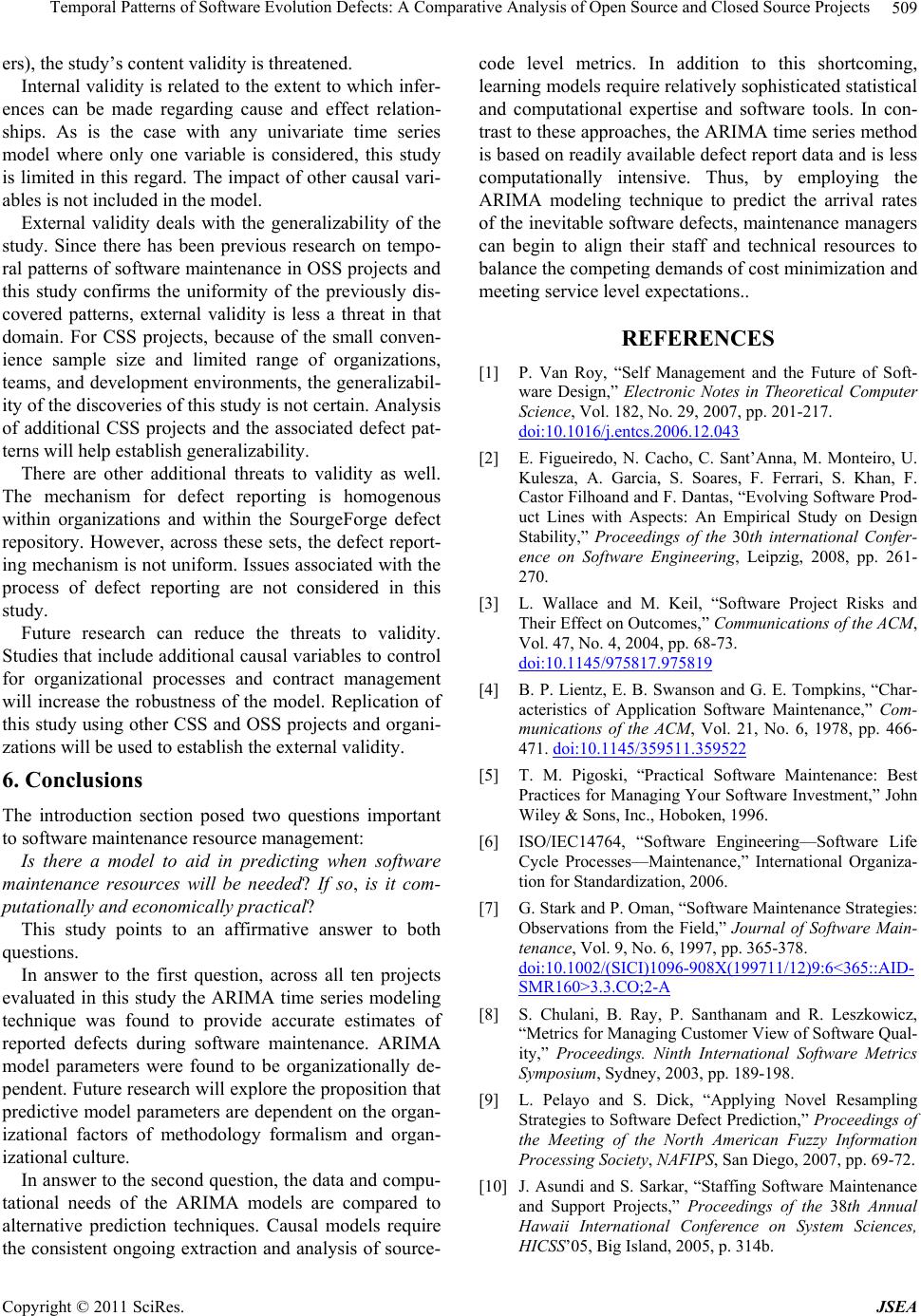 Temporal Patterns of Software Evolution Defects: A Comparative Analysis of Open Source and Closed Source Projects509 ers), the study’s content validity is threaten ed. Internal validity is related to the extent to which infer- ences can be made regarding cause and effect relation- ships. As is the case with any univariate time series model where only one variable is considered, this study is limited in this regard. The impact of other causal vari- ables is not included in the model. External validity deals with the generalizability of the study. Since there has been previous research on tempo- ral patterns of softwa re maintena nce in OSS projects and this study confirms the uniformity of the previously dis- covered patterns, external validity is less a threat in that domain. For CSS projects, because of the small conven- ience sample size and limited range of organizations, teams, and development environments, the gen eralizabil- ity of the discoveries of this study is not certain. Analysis of additional CSS projects and the associated defect pat- terns will help establish generalizability. There are other additional threats to validity as well. The mechanism for defect reporting is homogenous within organizations and within the SourgeForge defect repository. However, across these sets, the defect report- ing mechanism is not unifo rm. Issues associated with the process of defect reporting are not considered in this study. Future research can reduce the threats to validity. Studies that include additional causal v ariab les to contro l for organizational processes and contract management will increase the robustness of the model. Replication of this study using other CSS and OSS projects and organi- zations will be used to establish the external validity. 6. Conclusions The introduction section posed two questions important to software maintenance resource management: Is there a model to aid in predicting when software maintenance resources will be needed? If so, is it com- putationally and economically practical? This study points to an affirmative answer to both questions. In answer to the first question, across all ten projects evaluated in this study the ARIMA time series modeling technique was found to provide accurate estimates of reported defects during software maintenance. ARIMA model parameters were found to be organizationally de- pendent. Future research will explore the proposition that predictive model parameters are dependent on the organ- izational factors of methodology formalism and organ- izational culture. In answer to the second question, the data and compu- tational needs of the ARIMA models are compared to alternative prediction techniques. Causal models require the consistent ongoing extraction and analysis of source- code level metrics. In addition to this shortcoming, learning models require relatively sophisticated statistical and computational expertise and software tools. In con- trast to these approaches, the ARIMA time series method is based on readily available defect report data and is less computationally intensive. Thus, by employing the ARIMA modeling technique to predict the arrival rates of the inevitable software defects, maintenance managers can begin to align their staff and technical resources to balance the competing demands of cost minimization and meeting service level expectations.. REFERENCES [1] P. Van Roy, “Self Management and the Future of Soft- ware Design,” Electronic Notes in Theoretical Computer Science, Vol. 182, No. 29, 2007, pp. 201-217. doi:10.1016/j.entcs.2006.12.043 [2] E. Figueiredo, N. Cacho, C. Sant’Anna, M. Monteiro, U. Kulesza, A. Garcia, S. Soares, F. Ferrari, S. Khan, F. Castor Filhoand and F. Dantas, “Evolving Software Prod- uct Lines with Aspects: An Empirical Study on Design Stability,” Proceedings of the 30th international Confer- ence on Software Engineering, Leipzig, 2008, pp. 261- 270. [3] L. Wallace and M. Keil, “Software Project Risks and Their Effect on Outcomes,” Communications of the ACM, Vol. 47, No. 4, 2004, pp. 68-73. doi:10.1145/975817.975819 [4] B. P. Lientz, E. B. Swanson and G. E. Tompkins, “Char- acteristics of Application Software Maintenance,” Com- munications of the ACM, Vol. 21, No. 6, 1978, pp. 466- 471. doi:10.1145/359511.359522 [5] T. M. Pigoski, “Practical Software Maintenance: Best Practices for Managing Your Software Investment,” John Wiley & Sons, Inc., Hoboken, 1996. [6] ISO/IEC14764, “Software Engineering—Software Life Cycle Processes—Maintenance,” International Organiza- tion for Standardization, 2006. [7] G. Stark and P. Oman, “Software Maintenance Strategies: Observations from the Field,” Journal of Software Main- tenance, Vol. 9, No. 6, 1997, pp. 365-378. doi:10.1002/(SICI)1096-908X(199711/12)9:6<365::AID- SMR160>3.3.CO;2-A [8] S. Chulani, B. Ray, P. Santhanam and R. Leszkowicz, “Metrics for Managing Customer View of Software Qual- ity,” Proceedings. Ninth International Software Metrics Symposium, Sydney, 2003, pp. 189-198. [9] L. Pelayo and S. Dick, “Applying Novel Resampling Strategies to Software Defect Prediction,” Proceedings of the Meeting of the North American Fuzzy Information Processing Society, NAFIPS, San Diego, 2007, pp. 69-72. [10] J. Asundi and S. Sarkar, “Staffing Software Maintenance and Support Projects,” Proceedings of the 38th Annual Hawaii International Conference on System Sciences, HICSS’05, Big Island, 2005, p. 314b. Copyright © 2011 SciRes. JSEA  Temporal Patterns of Software Evolution Defects: A Comparative Analysis of Open Source and Closed Source Projects 510 [11] T. Chan, “Beyond Productivity in Software Maintenance: Factors Affecting Lead Time in Servicing Users’ Re- quests,” Proceedings of the International Conference on Software Maintenance, San Jose, 2000, pp. 228-237. [12] G. Antoniol, M. Di Penta and E. Merlo, “An Automatic Approach to Identify Class Evolution Discontinuities,” Proceedings of the 7th International Workshop on Prin- ciples of Software Evolution, Kyoto, 2004, pp. 31-40. doi:10.1109/IWPSE.2004.1334766 [13] M. C. Ohlsson, A. Amschler Andrews and C. Wohlin, “Modelling Fault-Proneness Statistically over a Sequence of Releases: A Case Study,” Journal of Software Main- tenance, Vol. 13, No. 3, 2001, pp. 167-199. doi:10.1002/smr.229 [14] T. M. Khoshgoftaar and D. L. Lanning, “A Neural Net- work Approach for Early Detection of Program Modules Having High Risk in the Maintenance Phase,” Journal of Systems and Software, Vol. 29, No. 2, 1995, pp. 85-91. doi:10.1016/0164-1212(94)00130-F [15] K. El-Emam and O. Laitenberger, “Evaluating Capture- Recapture Models with Two Inspectors,” IEEE Transac- tions on Software Engineering, Vol. 27, No. 9, 2001, pp. 851-864. doi:10.1109/32.950319 [16] T. M. Khoshgoftaar, B. Bhattacharyya and G. Richardson, “Predicting Software Errors, During Development, Using Nonlinear Regression Models: A Comparative Study,” IEEE Transactions on Reliability, Vol. 41, No. 3, 1992, pp. 390-395. doi:10.1109/24.159804 [17] N. E. Fenton and M. Neil, “A Critique of Software Defect Prediction Models,” IEEE Transactions on Software En- gineering, 25, No. 5, 1999, pp. 675-689. doi:10.1109/32.815326 [18] E. N. Adams, “Optimizing Preventive Service of Soft- ware Products,” IBM Journal of Research and Develop- ment, Vol. 28, No. 1, 1984, pp. 2-14. doi:10.1147/rd.281.0002 [19] M. S. Krishnan and M. I. Kellner, “Measuring Process Consistency: Implications for Reducing Software De- fects,” IEEE Transactions on Software Engineering, Vol. 25, No. 6, 1999, pp. 800-815. doi:10.1109/32.824401 [20] M. S. Krishnan, “The Role of Team Factors in Software Cost and Quality: An Empirical Analysis,” Information Technology & People, Vol. 11, No. 1, 1998, pp. 20-35. doi:10.1108/09593849810204512 [21] M. Hecht and J. Handal, “A Discrete-Event Simulator for Predicting Outage Time and Costs as a Function of Main- tenance Resources,” Reliability and Maintainability Sym- posium Proceedings. Annual, Seattle, 2002, pp. 612-617. [22] M. M. T. Thwin and T.-S. Quah, “Application of Neural Networks for Software Quality Prediction Using Object- Oriented Metrics,” Journal System and Software, Vol. 76, No. 2, 2005, pp. 147-156. doi:10.1016/j.jss.2004.05.001 [23] A. Tsakonas and G. Dounias, “Predicting Defects in Software Using Grammar-Guided Genetic Program- ming,” Proceedings of the 5th Hellenic conference on Ar- tificial Intelligence, SETN, Syros, 2008, pp. 413-418. [24] S. Dick and A. Sadia, “Fuzzy Clustering of Open-Source Software Quality Data: A Case Study of Mozilla,” IJCNN ’06. International Joint Conference on Neural Networks, Vancouver, 2006, pp. 4089-4096. doi:10.1109/IJCNN.2006.246954 [25] T. M. Khoshgoftaar, E. B. Allen, W. D. Jones and J. I. Hudepohl, “Classification Tree Models of Software Qual- ity over Multiple Releases,” Proceedings. 10th Interna- tional Symposium in Software Reliability Engineering, IEEE Reliability Society, 1999, pp. 116-125. [26] N. Seliya, T. M. Khoshgoftaar and S. Zhong, “Analyzing Software Quality with Limited Fault-Proneness Defect Data,” Ninth IEEE International Symposium on High- Assurance Systems Engineering, HASE, Heidelberg, 2005, pp. 89-98. [27] H. Zhang, S. Jarzabek and B. Yang, “Quality Prediction and Assessment for Product Lines,” Proceedings of the 15th International Conference on Advanced Information Systems Engineering, Klagenfurt, 2003, pp. 681-695. [28] T. Menzies, J. Greenwald and A. Frank, “Data Mining Static Code Attributes to Learn Defect Predictors,” IEEE Transactions on Software Engineering, Vol. 32, No. 1, 2007, pp. 2-13. doi:10.1109/TSE.2007.256941 [29] V. U. B. Challagulla, F. B. Bastani, I.-L. Yen and R. A. Paul, “Empirical Assessment of Machine Lea rning Based Software Defect Prediction Techniques,” IEEE Int’l Workshop on Object-oriented Real-time Dependable Sys- tems (WORDS), Sedona, 2005, pp. 282-303. [30] Q. Song, M. Shepperd, M. Cartwright and C. Mair, “Software Defect Association Mining and Defect Correc- tion Effort Prediction,” IEEE Transactions on Software Engineering, Vol. 32, No. 2, 2006, pp. 69-82. doi:10.1109/TSE.2006.1599417 [31] S. H. Aljahdali, A. Sheta and D. Rine, “Prediction of Software Reliability: A Comparison between Regression and Neural Network Non-Parametric Models,” ACS/IEEE International Conference on Computer Systems and Ap- plications, Beirut, 2001, pp. 470-473. doi:10.1109/AICCSA.2001.934046 [32] W. S. Humphrey and N. D. Singpurwalla, “Predicting (Individual) Software Productivity,” IEEE Transactions on Software Engineering, Vol. 17, No. 2, 1991, pp. 196- 207. doi:10.1109/32.67600 [33] A. Mital, A. Desai, A. Subramanian and A. Mital, “Prod- uct Development: A Structured Approach to Consumer Product Development, Design, and Manufacture,” But- terworth-Heinemann, 2008. [34] P. H. Franses, “Periodicity and Stochastic Trends in Eco- nomic Time Series,” Oxford University Press, Oxford, 1996. [35] E. Ghysels and D. R. Osborn, “The Econometric Analysis of Seasonal Time Series,” Cambridge University Press, Cambridge, 2001. [36] U. Raja, D. P. Hale and J. E. Hale, “Modeling Software Evolution Defects: A Time Series Approach,” Journal of Software Maintenance and Evolution: Research and Practice, Vol. 21, No. 6, 2009, pp. 49-71. doi:10.1002/smr.398 Copyright © 2011 SciRes. JSEA  Temporal Patterns of Software Evolution Defects: A Comparative Analysis of Open Source and Closed Source Projects Copyright © 2011 SciRes. JSEA 511 [37] C. F. Kemerer and S. A. Slaughter, “A Longitudinal Analysis of Software Maintenance Patterns,” ICIS Inter- national Conference on Information Systems Proceedings of the eighteenth ICIS, Atlanta, 1997, pp. 476-477. [38] B. Kenmei, G. Antoniol and M. Di Penta, “Trend Analy- sis and Issue Prediction in Large-Scale Open Source Sys- tems,” 12th European Conference on Software Mainte- nance and Reengineering, CSMR. 2008, pp. 73-82. [39] C. Chatfield, “The Analysis of Time Series: An Introduc- tion (6th Edition),” Chapman and Hall/CRC, London, 2003. [40] G. Box and G. Jenkins, “Time Series Analysis: Forecast- ing and Control,” Holden-Day, San Francisco, 1970. [41] R. R. Picard and R. D. Cook, “Cross-Validation of Re- gression Models,” Journal of the American Statistical Association, Vol. 79, No. 387, 1984, pp. 575-583. doi:10.2307/2288403 [42] I. Herraiz, J. M. Gonzalez-Barahona, G. Robles and D. M. German, “On the Prediction of the Evolution of Libre Software Projects,” IEEE International Conference on Software Maintenance, (ICSM 2007), Paris, 2007, pp. 405-414. doi:10.1109/ICSM.2007.4362653 [43] G. M. Ljung and G. E. P. Box, “On a Measure of Lack of fit in Time Series Models,” Biometrika Trust, Vol. 65, No. 2, 1978, pp. 297-303. doi:10.1093/biomet/65.2.297 [44] K. Gregory, “Native-View Paradigms: Multiple Cultures and Culture Conflicts in Organizations,” Administrative Science Quarterly, Vol. 28, No. 3, 1983, pp. 359-376. doi:10.2307/2392247 [45] D. Thomas, “Hacker Culture,” University of Minnesota Press, Minneapolis, 2003. [46] K. Crowston and B. Scozzi, “Open Source Software Pro- jects as Virtual Organisations: Competency Rallying for Software Development,” IEE Proceedings Software, Vol. 149, 2002, pp. 3-17. doi:10.1049/ip-sen:20020197 [47] T. T. Dinh-Trong and J. M. Bieman, “The FreeBSD Pro- ject: A Replication Case Study of Open Source Develop- ment,” IEEE Transactions on Software Engineering, Vol. 31, No. 6, 2005, pp. 481-494. doi:10.1109/TSE.2005.73 [48] F. N. Kerlinger and H. B. Lee, “Foundations of Behav- ioral Research,” 4th Edition, Wadsworth, New York, 1999.
|