Smart Grid and Renewable Energy, 2011, 2, 190-205
doi:10.4236/sgre.2011.23023 Published Online August 2011 (http://www.SciRP.org/journal/sgre)
Energy, Exergy and Thermoeconomics Analysis of
Water Chiller Cooler for Gas Turbines Intake Air
Cooling
Galal Mohammed Zaki1, Rahim Kadhim Jassim2, Majed Moalla Alhazmy1
1Department of Thermal Engineering and Desalination Technology, King Abdulaziz University, Jeddah, Saudi Arabia; 2Department
of Mechanical Engineering Technology, Yanbu Industrial College, Yanbu Industrial City, Saudi Arabia.
Received June 24, 2010; revised May 23, 2011; accepted May 30, 2011.
ABSTRACT
Gas turbine (GT) power plants operating in arid climates suffer a decrease in output power during the hot summer
months because of the high specific volume of air drawn by the compressor. Cooling the air intake to the compressor
has been widely used to mitigate this shortcoming. Energy and exergy analysis of a GT Brayton cycle coupled to a re-
frigeration air cooling unit shows a promise for increasing the output power with a little decrease in thermal efficiency.
A thermo-economics algorithm is developed to estimate the economic feasibility of the cooling system. The analysis is
applied to an open cycle, HITACHI-FS7001B GT plant at the industrial city of Yanbu (Latitude 24˚05" N and longitude
38˚ E) by the Red Sea in the Kingdom of Saudi Arabia. Result show that the enhancement in output power depends on
the degree of chilling the air intake to the compressor (a 12 - 22 K decrease is achieved). For this case study, maximum
power gain ratio (PGR) is 15.46% (average of 12.25%), at an insignificant decrease in thermal efficiency. The second
law analysis show that the exergetic power gain ratio drops to an average 8.5%. The cost of adding the air cooling sys-
tem is also investigated and a cost function is derived that incorporates time-dependent meteorological data, operation
characteristics of the GT and the air intake cooling system and other relevant parameters such as interest rate, lifetime,
and operation and maintenance costs. The profit of adding the air cooling system is calculated for different electricity
tariff.
Keywords: Gas Turbine, Exergy Analysis, Power Boosting, Hot Climate, Air cooling, Water Chiller
1. Introduction
During hot summer months, the demand for electricity
increases and utilities may experience difficulty meeting
the peak loads, unless they have sufficient reserves. In all
Gulf States, where the weather is fairly hot year around,
air conditioning (A/C) is a driving factor for electricity
demand and operation schedules. The utilities employ
gas turbine (GT) power plants to meet the A/C peak load.
Unfortunately, the power output and thermal efficiency
of GT plants decrease in the summer because of the in-
crease in the compressor power. The lighter hot air at the
GT intake decreases the mass flow rate and in turn the
net output power. For an ideal GT open cycle, the de-
crease in the net output power is –0.4% for every 1 K
increase in the ambient air temperature. To overcome this
problem, air intake cooling methods, such as evaporative
(direct method) and/or refrigeration (indirect method) has
been widely considered [1].
In the direct method of evaporative cooling, the air in-
take cools off by contacts with a cooling fluid, such as
atomized water sprays, fog or a combination of both, [2].
Evaporative cooling has been extensively studied and
successfully implemented for cooling the air intake in
GT power plants in dry hot regions [3-7]. This cooling
method is not only simple and inexpensive, but the water
spray also reduces the NOx content in the exhaust gases.
Recently, Sanaye and Tahani [8] investigated the effect
of using a fog cooling system, with 1 and 2% over-spray,
on the performance of a combined GT; they reported an
improvement in the overall cycle heat rate for several GT
models. Although evaporative cooling systems have low
capital and operation cost, reliable and require moderate
maintenance, they have low operation efficiency, con-
sume large quantities of water and the impact of the non
evaporated water droplets in the air stream could damage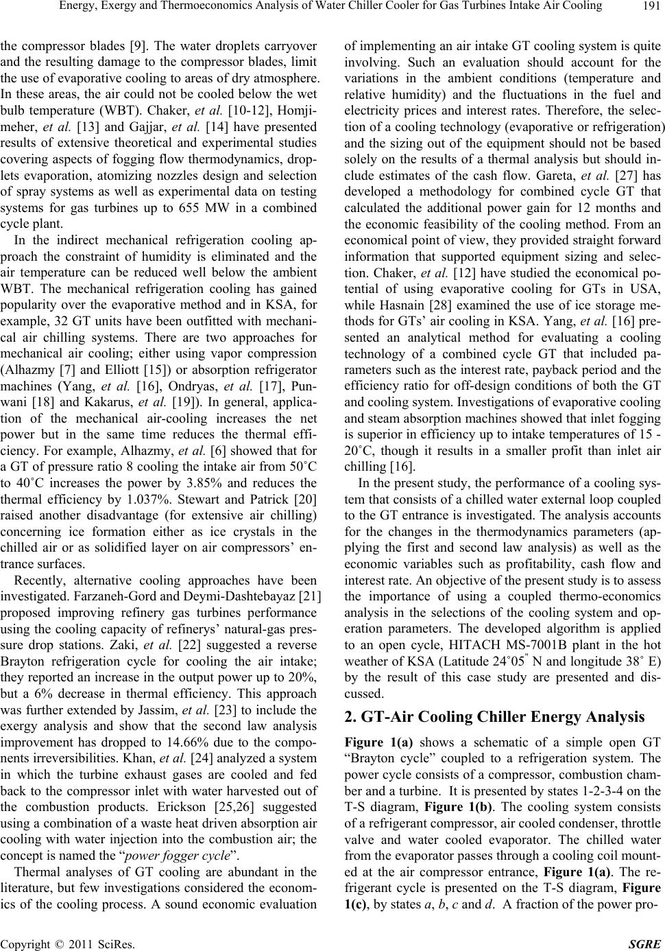

Energy, Exergy and Thermoeconomics Analysis of Water Chiller Cooler for Gas Turbines Intake Air Cooling191
the compressor blades [9]. The water droplets carryover
and the resulting damage to the compressor blades, limit
the use of evaporative cooling to areas of dry atmosphere.
In these areas, the air could not be cooled below the wet
bulb temperature (WBT). Chaker, et al. [10-12], Homji-
meher, et al. [13] and Gajjar, et al. [14] have presented
results of extensive theoretical and experimental studies
covering aspects of fogging flow thermodynamics, drop-
lets evaporation, atomizing nozzles design and selection
of spray systems as well as experimental data on testing
systems for gas turbines up to 655 MW in a combined
cycle plant.
In the indirect mechanical refrigeration cooling ap-
proach the constraint of humidity is eliminated and the
air temperature can be reduced well below the ambient
WBT. The mechanical refrigeration cooling has gained
popularity over the evaporative method and in KSA, for
example, 32 GT units have been outfitted with mechani-
cal air chilling systems. There are two approaches for
mechanical air cooling; either using vapor compression
(Alhazmy [7] and Elliott [15]) or absorption refrigerator
machines (Yang, et al. [16], Ondryas, et al. [17], Pun-
wani [18] and Kakarus, et al. [19]). In general, applica-
tion of the mechanical air-cooling increases the net
power but in the same time reduces the thermal effi-
ciency. For example, Alhazmy, et al. [6] showed that for
a GT of pressure ratio 8 cooling the intake air from 50˚C
to 40˚C increases the power by 3.85% and reduces the
thermal efficiency by 1.037%. Stewart and Patrick [20]
raised another disadvantage (for extensive air chilling)
concerning ice formation either as ice crystals in the
chilled air or as solidified layer on air compressors’ en-
trance surfaces.
Recently, alternative cooling approaches have been
investigated. Farzaneh-Gord and Deymi-Dashtebayaz [21]
proposed improving refinery gas turbines performance
using the cooling capacity of refinerys’ natural-gas pres-
sure drop stations. Zaki, et al. [22] suggested a reverse
Brayton refrigeration cycle for cooling the air intake;
they reported an increase in the output power up to 20%,
but a 6% decrease in thermal efficiency. This approach
was further extended by Jassim, et al. [23] to include the
exergy analysis and show that the second law analysis
improvement has dropped to 14.66% due to the compo-
nents irreversibilities. Khan, et al. [24] analyzed a system
in which the turbine exhaust gases are cooled and fed
back to the compressor inlet with water harvested out of
the combustion products. Erickson [25,26] suggested
using a combination of a waste heat driven absorption air
cooling with water injection into the combustion air; the
concept is named the “power fogger cycle”.
Thermal analyses of GT cooling are abundant in the
literature, but few investigations considered the econom-
ics of the cooling process. A sound economic evaluation
of implementing an air intake GT cooling system is quite
involving. Such an evaluation should account for the
variations in the ambient conditions (temperature and
relative humidity) and the fluctuations in the fuel and
electricity prices and interest rates. Therefore, the selec-
tion of a cooling technology (evaporative or refrigeration)
and the sizing out of the equipment should not be based
solely on the results of a thermal analysis but should in-
clude estimates of the cash flow. Gareta, et al. [27] has
developed a methodology for combined cycle GT that
calculated the additional power gain for 12 months and
the economic feasibility of the cooling method. From an
economical point of view, they provided straight forward
information that supported equipment sizing and selec-
tion. Chaker, et al. [12] have studied the economical po-
tential of using evaporative cooling for GTs in USA,
while Hasnain [28] examined the use of ice storage me-
thods for GTs’ air cooling in KSA. Yang, et al. [16] pre-
sented an analytical method for evaluating a cooling
technology of a combined cycle GT that included pa-
rameters such as the interest rate, payback period and the
efficiency ratio for off-design conditions of both the GT
and cooling system. Investigations of evaporative cooling
and steam absorption machines showed that inlet fogging
is superior in efficiency up to intake temperatures of 15 -
20˚C, though it results in a smaller profit than inlet air
chilling [16].
In the present study, the performance of a cooling sys-
tem that consists of a chilled water external loop coupled
to the GT entrance is investigated. The analysis accounts
for the changes in the thermodynamics parameters (ap-
plying the first and second law analysis) as well as the
economic variables such as profitability, cash flow and
interest rate. An objective of the present study is to assess
the importance of using a coupled thermo-economics
analysis in the selections of the cooling system and op-
eration parameters. The developed algorithm is applied
to an open cycle, HITACH MS-7001B plant in the hot
weather of KSA (Latitude 24˚05" N and longitude 38˚ E)
by the result of this case study are presented and dis-
cussed.
2. GT-Air Cooling Chiller Energy Analysis
Figure 1(a) shows a schematic of a simple open GT
“Brayton cycle” coupled to a refrigeration system. The
power cycle consists of a compressor, combustion cham-
ber and a turbine. It is presented by states 1-2-3-4 on the
T-S diagram, Figure 1(b). The cooling system consists
of a refrigerant compressor, air cooled condenser, throttle
valve and water cooled evaporator. The chilled water
from the evaporator passes through a cooling coil mount-
ed at the air compressor entrance, Figure 1(a). The re-
frigerant cycle is presented on the T-S diagram, Figure
1(c), by states a, b, c and d. A fraction of the power pro-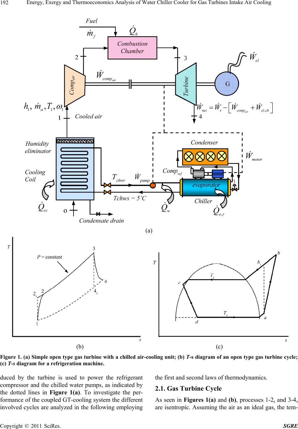

Energy, Exergy and Thermoeconomics Analysis of Water Chiller Cooler for Gas Turbines Intake Air Cooling 192
(a)
(b) (c)
Figure 1. (a) Simple open type gas turbine with a chilled air-cooling unit; (b) T-s diagram of an open type gas turbine cycle;
(c) T-s diagram for a refrigeration machine.
duced by the turbine is used to power the refrigerant
compressor and the chilled water pumps, as indicated by
the dotted lines in Figure 1(a). To investigate the per-
formance of the coupled GT-cooling system the different
involved cycles are analyzed in the following employing
the first and second laws of thermodynamics.
2.1. Gas Turbine Cycle
As seen in Figures 1(a) and (b), processes 1-2s and 3-4s
are isentropic. Assuming the air as an ideal gas, the tem-
C
opyright © 2011 SciRes. SGRE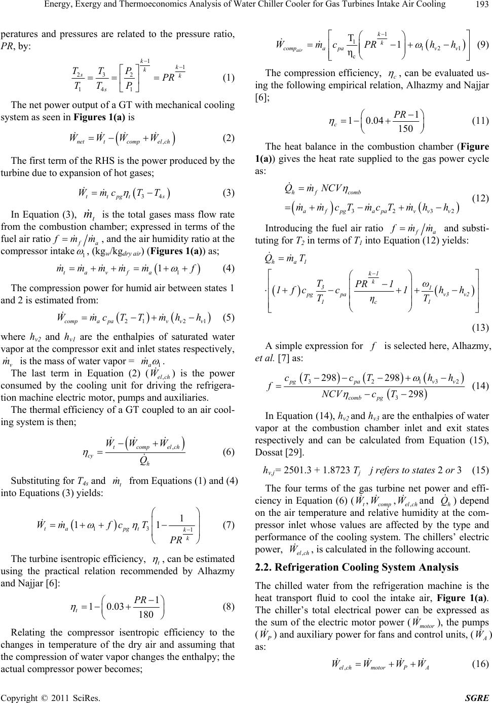

Energy, Exergy and Thermoeconomics Analysis of Water Chiller Cooler for Gas Turbines Intake Air Cooling193
peratures and pressures are related to the pressure ratio,
PR, by:
1
1
23 2
14 1
k
k
k
sk
s
TT PPR
TT P


 

 (1)
The net power output of a GT with mechanical cooling
system as seen in Figures 1(a) is

,nettcompel ch
WWW W 
 


(2)
The first term of the RHS is the power produced by the
turbine due to expansion of hot gases;

34ttpgt s
Wmc TT  
 (3)
In Equation (3), t is the total gases mass flow rate
from the combustion chamber; expressed in terms of the
fuel air ratio
m

f
a
f
mm
1
, and the air humidity ratio at the
compressor intake

, (kgw/kgdry air) (Figures 1(a)) as;

1
1
tavf a
mmmm mf   


(4)
The compression power for humid air between states 1
and 2 is estimated from:
 
212 1compa pavvv
WmcTTmhh

(5)
where hv2 and hv1 are the enthalpies of saturated water
vapor at the compressor exit and inlet states respectively,
is the mass of water vapor =
v
m
1a
m



.
The last term in Equation (2) (,el ch
W) is the power
consumed by the cooling unit for driving the refrigera-
tion machine electric motor, pumps and auxiliaries.
The thermal efficiency of a GT coupled to an air cool-
ing system is then;


,tcompelch
cy
h
WW W
Q



 
 (6)
Substituting for T4s and from Equations (1) and (4)
into Equations (3) yields:
t
m


13
1
1
11
tapgtk
k
Wmfc T
PR




 




(7)
The turbine isentropic efficiency, t

, can be estimated
using the practical relation recommended by Alhazmy
and Najjar [6]:
1
10.03180
t
PR



 




actual compressor power becomes;
(8)
Relating the compressor isentropic efficiency to the
changes in temperature of the dry air and assuming that
the compression of water vapor changes the enthalpy; the

1
1
Tk
k

12 1
c
1
η
air
comp a pavv
WmcPR hh 













 (9)
The compression efficiency,

c

, can be evaluated us-
ing the following empirical relat, Alhazmy and Najjar
[6];
ion
1
10.04 150
c
PR



 


(11)
The heat balance in the combustion chamber (
1(
2
(12)
Introducing the fuel air ratio
Figure
a)) gives the heat rate supplied to the gas power cycle
as:


323
hf comb
afpg apa vvv
Qm NCV
mmcTmcTmh h
 
 

 
f
a
f
mm and substi-
tu quation (12ting for T2 in terms of T1 into E) yields:
 
ha1
QmT

k1
k
31
pg pav3 v2
1c1
Tω PR 1
1fcc1h h
TηT




 
 

 






(13)
A simple expression for

f
is selected here, Alha
et
zmy,
al. [7] as:



 

3213
3
298 298
298
pgpav v
comb pg
2
cTh h
fNCV c T


  
 (14)
In Equation (14), hv2 and hv3 are the enthalpies of water
va i
+ 1.8723 Tj j refers to states 2 or 3 (15)
ci
is the
cT
por at the combuston chamber inlet and exit states
respectively and can be calculated from Equation (15),
Dossat [29].
hv,j= 2501.3
The four terms of the gas turbine net power and effi-
ency in Equation (6) (,
tcomp
WW
 ,,el ch
W
and h
Q
) depend
on the air temperature aneidity the com-
pressor inlet whose values are affected by the type and
performance of the cooling system. The chillers’ electric
power, ,el ch W
, is calculated in the following account.
2.2. Refrigeration Cooling System Analysis
d relativ humat
The chilled water from the refrigeration machine
heat transport fluid to cool the intake air, Figure 1(a).
The chiller’s total electrical power can be expressed as
the sum of the electric motor power (motor
W
), the pumps
(
P
W
) and auxiliary power for fans and control units, (A
W
)
as:
,el chmotorPA
WWWW
  
(16)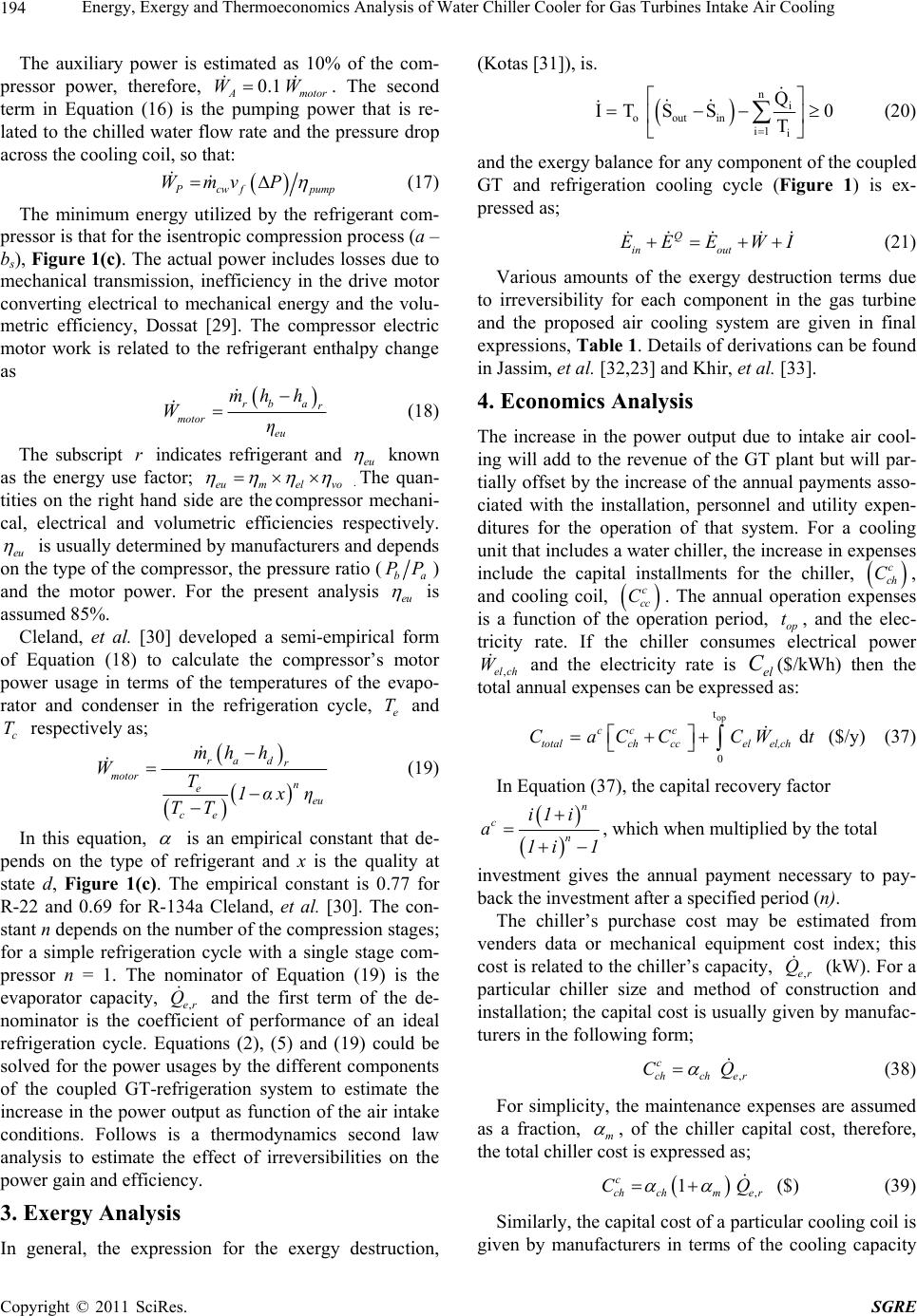

Energy, Exergy and Thermoeconomics Analysis of Water Chiller Cooler for Gas Turbines Intake Air Cooling 194
The auxiliary power is estimated as 10%
press
of the com-
or power, therefore, 0.1
A motor
WW. The second
term in Equation (16) is the pumping power that is re-
lated to the chilled water flow rate and the pressure drop
across the cooling coil, so that:



P
cw f
Wmv P  
 (17)
pump
The minimum energy utilized by the ref
press
rigerant com-
or is that for the isentropic compression process (a –
bs), Figure 1(c) . The actual power includes losses due to
mechanical transmission, inefficiency in the drive motor
converting electrical to mechanical energy and the volu-
metric efficiency, Dossat [29]. The compressor electric
motor work is related to the refrigerant enthalpy change
as

rb a
r
motor
eu
mh h

Wη 
 (18)
The subscript indicates refrigerant an r d eu

known
as the fact energy useor; eum el vo



 .
tities on the right hand side are the compressor mechani-
cal, electrical and volumetric effiespectively.
eu
The quan-
ciencies r

is usually determined by manufacturers and depends
on the type of the compressor, the pressure ratio (ba
PP)
and the motor power. For the present analysis eu

is
assumed 85%.
Cleland, et al. [30] developed a semi-empiricalrm
of Equation (1
fo
8) to calculate the compressor’s motor
power usage in terms of the temperatures of the evapo-
rator and condenser in the refrigeration cycle, e
T and
c
T respectively as;



rad
r
motor
mh h
W 

n
e
eu
ce
T1αxη
TT  
(19)
In this equation,

is an empirical constant that de-
pen
on for the exergy destruction,
ds on the type of refrigerant and x is the quality at
state d, Figure 1(c). The empirical constant is 0.77 for
R-22 and 0.69 for R-134a Cleland, et al. [30]. The con-
stant n depends on the number of the compression stages;
for a simple refrigeration cycle with a single stage com-
pressor n = 1. The nominator of Equation (19) is the
evaporator capacity, ,er
Q
 and the first term of the de-
nominator is the coefficient of performance of an ideal
refrigeration cycle. Equations (2), (5) and (19) could be
solved for the power usages by the different components
of the coupled GT-refrigeration system to estimate the
increase in the power output as function of the air intake
conditions. Follows is a thermodynamics second law
analysis to estimate the effect of irreversibilities on the
power gain and efficiency.
3. Exergy Analysis
In general, the expressi
(Kotas [31]), is.

n
i
ooutin
i1 i
Q
IT SS0
T








 (20)
and the exergy balance for any component of the coupled
GT and refrigeration cooling cycle (Figure 1) is ex-
pressed as;
Q
in out
EE E WI


  
(21)
Various amounts of the exergy destru
to
tput due to intake air cool-
ction terms due
irreversibility for each component in the gas turbine
and the proposed air cooling system are given in final
expressions, Table 1. Details of derivations can be found
in Jassim, et al. [32,23] and Khir, et al. [33].
4. Economics Analysis
The increase in the power ou
ing will add to the revenue of the GT plant but will par-
tially offset by the increase of the annual payments asso-
ciated with the installation, personnel and utility expen-
ditures for the operation of that system. For a cooling
unit that includes a water chiller, the increase in expenses
include the capital installments for the chiller,


c
ch
C,
and cooling coil,


c
cc
C. The annual operation exp
is a function of thration period, op
t, and the elec-
tricity rate. If the chiller consumes electrical power
,el ch
W
 and the electricity rate is el
C($/kWh) then the
nnual expenses can be expresas:
op
t
enses
e ope
total ased
0
d
cc c
totalchccel el,ch
CaCC CW



 t($/y) (37)
In Equation (37), the capital recovery factor


n
i1 i
c
n
a
1i 1


, which when multiplied by the total
investment gives the annual payment necessary to pay-
ed from
ve
Q (38)
For simplicity, the maintenance expe
as
back the investment after a specified period (n).
The chiller’s purchase cost may be estimat
nders data or mechanical equipment cost index; this
cost is related to the chiller’s capacity, ,er
Q
 (kW). For a
particular chiller size and method of ruction and
installation; the capital cost is usually given by manufac-
turers in the following form;
c
C  
const
, ch che r

nses are assumed
a fraction, m

, of the chiller capital cost, therefore,
the total chillerst is expressed as; co


1
c
CQ  
,ch chme r ($) (39)
Similarly, the capital cost of a particu
gi
lar cooling coil is
ven by manufacturers in terms of the cooling capacity
C
opyright © 2011 SciRes. SGRE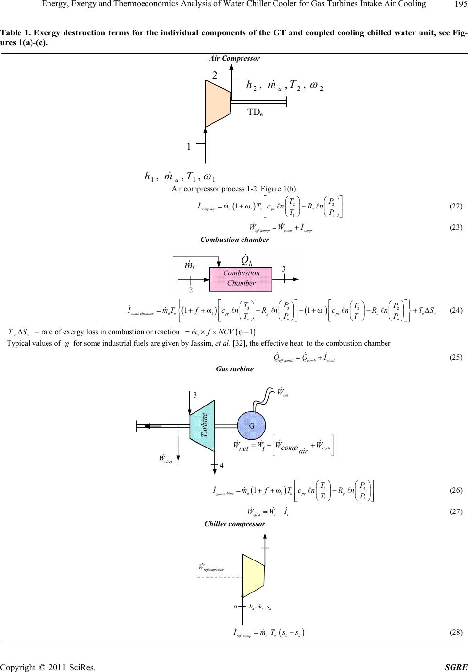

Energy, Exergy and Thermoeconomics Analysis of Water Chiller Cooler for Gas Turbines Intake Air Cooling 195
nts of the GT and coupled cooling chilled water unit, see Fig-
Air Compressor
Table 1. Exergy destruction terms for the individual compone
ures 1(a)-(c).
TD
e
1
111 ,,,
 Tmh a

2
222 ,,,
 Tmh a

Air compressor process 1-2, Figure 1(b).

2
1T ImωTc n2
,
11
comp aira1opaa
P
R n
TP


 




  
 

 (22)
(23)
Combustion chamber

,eff compcompcomp
WWI

 
33 22
11
1ω1ω
combchamberaopggpaaoo
oo oo
TP TP
I
mTfcnRncnRn T
TP TP


 


 
 

  


S





(24)
= rate of exergy loss in combustion or reaction
oo
TS


φ1
a
mfNCV

 

Typical values of

 for some industrial fuels are given by Jassim, et al. [32], the effective heat to the combustion chamber
(25)
Gas turbine
,eff combcombcomb
QQI
 

44
1
3
1ω
gas turbineaopgg
TP
ImfTcnRn
T3 P


 
 


 


 


 (26)
I
,eff ttt
WW



(27)
Chiller compressor

ref comprbao
I
mT ss
 (2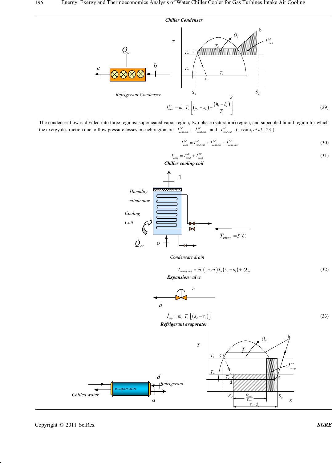8)

Energy, Exergy and Thermoeconomics Analysis of Water Chiller Cooler for Gas Turbines Intake Air Cooling 196
Chiller Condenser
R
efrigerant Condense
r
b
c
o
Q
S

T
o
b
3
S

2
S

T
cond
I

T
T
w
T
c
c
d
T
e
o
Q




Tb
condr ocb
o
hh
ImTss T
c







 (29)
The condenser flow is divided into three regions: superheated vapor region, two phase (saturation) region, and subcooled liquid region for which
(30)
the exergy destruction due to flow pressure losses in each region are ,sup
P
cond
I
, ,
P
cond sat
I
 and ,
P
cond sub
I
. (Jassim, et al. [23])
P


,sup ,,
PPP
condcondcond satcond sub
III I
 

 
TP
condcond cond
I
II



Chiller cooling coil
(31)
Humidity
eliminator
Cooling
Coil
o
cc
Q

Condensate drain
T
chws
=5˚C
1
 
1o1
1ss
cooling coilaoout
I
mT   
 Q (32)
Expansion valve
c
d

exp rod c
ImTss




 (33)
Refrigerant evaporator
Chilled water
evaporator
R
efrigeran
t
d
a
S

T
o
b
d
S

a
S

T
evap
I

T
T
w
T
c
c
d
T
e
o
Q

wch
evap
T
Q

a
da SS  
C
opyright © 2011 SciRes. SGRE

Energy, Exergy and Thermoeconomics Analysis of Water Chiller Cooler for Gas Turbines Intake Air Cooling 197


Ta
evapr oad
sw
hh
ImTss T
d










 (34)
The refrigerant flow in the evaporator is divided into two regimes saturation (two phase) and superheated regions. The two phase (saturation)
region, and superheated vapor region for which the exergy destruction due to flow pressure losses in each region are see Khir,
et
al. [33]. The exergy destruction rate is the sum of the thermal and pressure loss terms for both regimes (Equations (35) and (36)) as,
,
P
evapsat
I
, ,sup
P
evap
I

TP
evapevapevap
I
II



(35)
sup
(36)
,,
PP P
evapevapsatevap
II I
 

 
that is directly proportional to the total heat transfer sur-
face area (
cooling coil to enter the air compressor intake at and
, Figure 1(a). Both and dpend the
illed water su
Wh
va the
rocmay
r
1
T
on
ess
, m2) Kotas [31]) as,
($) (40)
cc
A
1eω
ch
rate,
be t
trated i
ing c
1
T1 ω
po
pply temperature (Tchws) and mass flow
en the outer surface temperature of the

m
c
cccccc
CA  
cw
m
.
ea
n
oil gi
cooling coil falls below the dew point (corresponding to
the partial pressure of the water r)water vapor
condensates and leaves the air stream. This p
ted as a cooling-dehumidification process as illus-
Figure 3. Steady state heat balance of the cool-
ves;
In Equation (40), cc

and m depend on the type of
e cooling coil and material. For the present study and
cal Saudi market, cc
th
lo

= 30000 and m= 0.582 are
recommended (Yorltation [3bstituting
Equations (39) and (40) into Equation (37), assuming for
mplicity that the chiller power is an average constant
nn
he
k Co consu4]). Su
si
value and constant electricity rate over the operation pe-
riod, the aual total expenses for the cooling system
become;


1ccaow wcw
Qmhhmhm


w chwr
T

1
c
totalchme rccccopelelch
CaQA tCW  




m

,,

( $/y) (41)
In Equation (41) the at transfer area cc

ris the chilledr
water extractiofrom th
,chws
T
eff cc
c 
mass flow
e air,
(45)
ate and w m  whe
is th
e, cw m 
e rate of
water
n


1wao
mm

 
. The second term in Equation (45) is
d can

be negl
usually a sm
ecte
ng
all term when cmp the first a
d, McQuiston, [35]
In Equation (45) the entalpy and temperature of the
o
et al.
h
ared to
.

n
air leavithe cooling coil (h1 and T1) may be calculated
from;

1oos
hhCFhh (46)

1oos
TTCFT (47)
The contact factor CF is defined as the ratio between
the actual air temperature drop to the maximum, at which
the air theatrically leaves at the coil surface temperature
Ts = Tchws and 100% relative humidity. Substituting for h1
from Equation (46) into Equation (45) and use Equation
(42) gives;
A
is the pa-
rameter used to evaluate the cost of the cooling coil. En-
ergy balance on both the cooling coil and the refrigerant
evaporator, taking into account the effectiveness factors
for the evaporator, ,eff er

, and the cooling coil, ,eff cc

,
gives
T
,,
,
ereff er
cc
cc
meffcc m
Q
Q
AUTFUTF







(4
where, U is the overall heat tran
ch G
coil
d chilled water fluids) is;


2)
sfer coefficient for
illed water-air tube bank heat exchanger. areta, et al.
[27] suggested a moderate value of 64 W/m2 K and 0.98
for the correction factor F.
Figure 2, illustrates the temperature variations in the
combined refrigerant, water chiller and air cooling sys-
tem. the mean temperature difference for the cooling
(air an

 
1

 
1
1
ochwr chws
nT TT T
Equations (40) and (42) give the cooling coil cost as,
o chwrchws
m
TT TT
T  
(43)
m
cQ
C 

cc
 (44)
cc cc
m
UT F



where, cc
Q
 is the thermal capacity of the cooling coil.
The atmospheric air enters at To and o

and leaves the
,
Q
,,
aochwso
er
r eff
mCFh h 

w
eff e
h
cc

 


 4)
s o
e
otal annual cotermv
, as,

n
t
er
Q

(
aporator ca-
8
Equatio (41) through (48) give the chiller and c
ing coil annual expenses in terms of the air mass flow
rate and propertis. The total annual cost function is de-
rived from Equation (41) as follows.
4.1. Annual Cost Function
o l-
Combining Equations (41) and (42), substituting for the
cooling coil surface area, pump and auxiliary power
gives thest in s of the e
pacity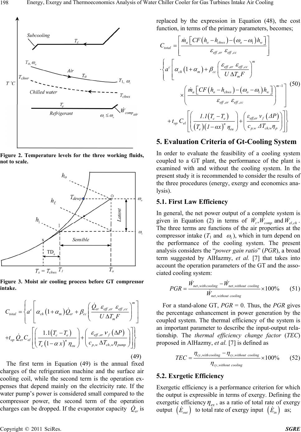

Energy, Exergy and Thermoeconomics Analysis of Water Chiller Cooler for Gas Turbines Intake Air Cooling 198
Figure 2. Temperature levels for the three working fluids,
not to scale.
Figure 3. Moist air cooling process before GT compressor
intake.




,,
,
,,
1ereff ereff cc
c
totalchm ercc
Ca QUTF  

 






1.1
1
m
m
eff erf
ce
oper eln
p wch wpump
eeu
Q
P
TT
tQC cT
Tx

















 














(49)
The first term in Equation (49) is the annual fixed
charges of the refrigeration machine and the surface air
cooling coil, while the second term is the operation ex-
penses that depend mainly on the electricity rate. If the
water pump’s power is considered small compared to the
compressor power, the second term of the operation
charges can be dropped. If the evaporator capacity is
replaced by the expression in Equation (48), the cost
function, in terms of the primary parameters, becomes;

er
Q





 
1
,,
,,
1
1
,,
1
aochwsow
total
eff ereffcc
m
eff ereff cc
c
chm cc
m
m
aochwsow
eff ereffcc
eff ,er
ce
mCFh hh
C
aUTF
mCFh hh
εν 1.1 TT
tC








 














 





op el n
eeu
T1αxη












fΔP





p,w ch,w p
cΔTη









(50)
5. Evaluation Criteria of Gt-Cooling System
In order to evaluate the feasibility of a cooling system
coupled to a GT plant, the performance of the plant is
examined with and without the cooling system. In t
present study it is recommended to consider the results of
the three procedures (energy, exergy and economics ana-
lysis).
5.1. First Law Efficiency
he
In general, the net power output of a complete system is
given in Equation (2) in terms of , ,and
tcomp elch
WW W
 .
The three terms are functions of the air properties at the
compressor intake (T1 and 1

), which in turn depend on
the performance of the cooling system. The present
analysis considers the “power gain ratio” (PGR), a broad
term suggested by AlHazmy, et al. [7] that takes into
account the operation parameters of the GT and the asso-
ciated cooling system:
,,
,
100%
net withcoolingnetwithout cooling
netwithout cooling
WW
PGR W



 (51)
For a stand-alone GT, PGR = 0. Thus, the PGR gives
the percentage enhancement in power generation by the
coupled system. The thermal efficiency of the syste
an important parameter to describe the input-output
tionship. The thermal efficiency change factor (TEC)
proposed in AlHazmy, et al. [7] is defined as
m is
rela-
,,
,
100%
cy withcoolingcy withoutcooling
cy without cooling
TEC




 (52)
5.2. Exrgetic Efficiency
Exergetic efficiency is a performance criterion for which
the output is expressible in terms of exergy. Defining the
exergetic efficiencyex
η, as a ratio of total rate of exergy
output


out
E
 to total rate of exergy input

in
E
 as;
C
opyright © 2011 SciRes. SGRE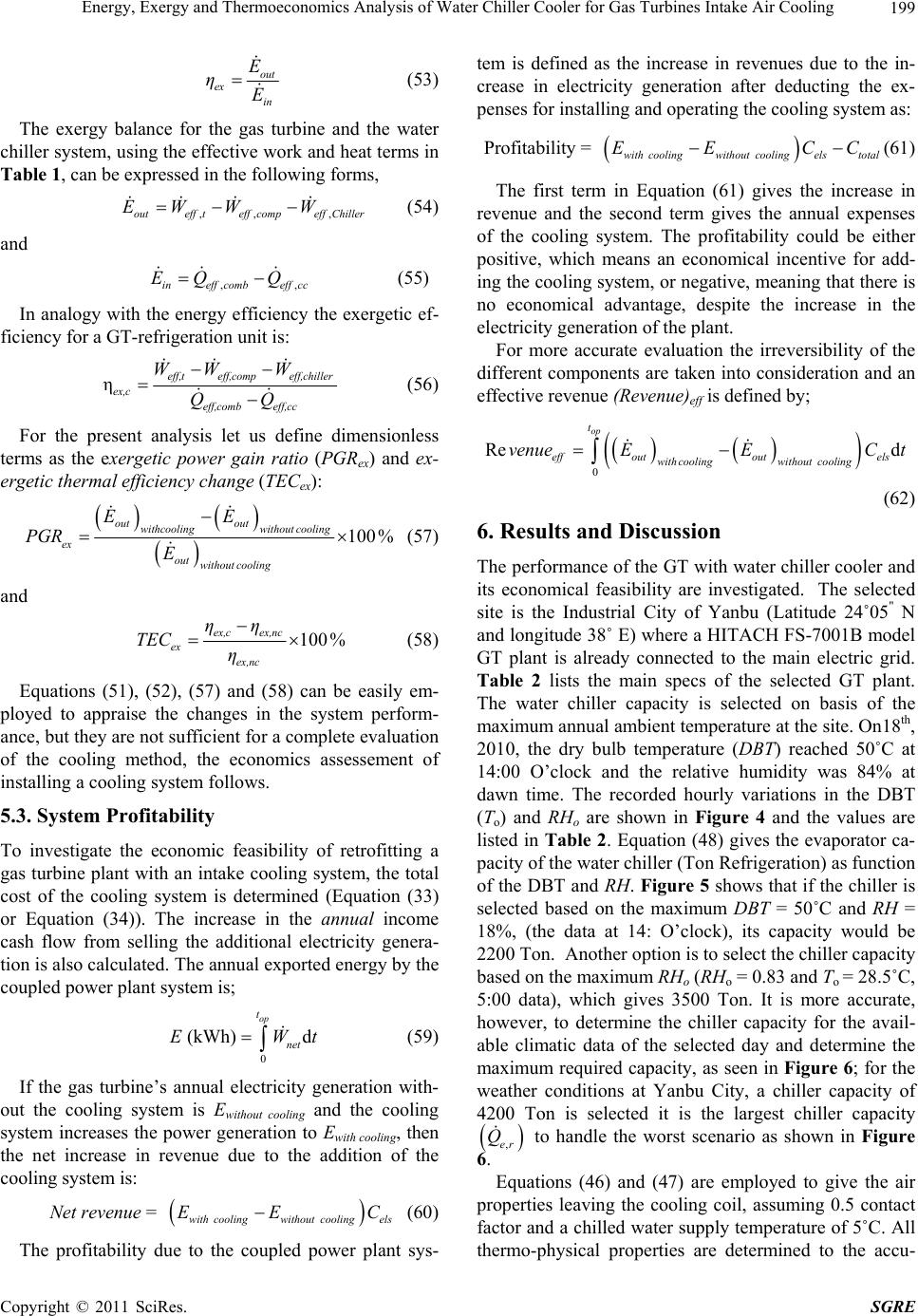

Energy, Exergy and Thermoeconomics Analysis of Water Chiller Cooler for Gas Turbines Intake Air Cooling199
out
ex
in
E
ηE 
 (53)
The exergy balance for the gas tu
chiller system, using the effec
rbine and the water
tive work and heat terms in
Table 1, can be expressed in the following forms,
,, ,outeff teff compeff Chiller
EW WW 
  (54)
and
,,ineff combeff cc
EQ Q
  (55)
In analogy with the energy efficiency the exergetic ef-
ficiency for a GT-refrigeration unit is:

ηeff,t eff,comp eff,chiller
ex,c
eff,comb eff,cc
W

W W
QQ


 
 (56)
For the present analysis let us define dimensionless
terms as the exergetic power gain ratio (PGRex) and ex-
ergetic thermal efficiency change (TECex):
 

100%
out out
withcoolingwithout cooling
ex
out withoutcooling
EE
PGR E



 (57)
and
100%
ex,cex,nc
ex
ex,nc
ηη
TEC η

 (58)
g a co
5.3. System Profitability
To investigate the economic feasibility of retrofitting a
ga
ncome
cash flow from selling the additional electricit
tion is also calculated. The annual exported ener
led power plant system is;
generation with-
out the cooling system is Ewithout cooling and the cooling
system increases the power generation to E
the net increase in revenue due to the addition of the
co
The profitability due to the coupled power plant sys-
tem is defined as the increase in revenues due to the in-
crease in electricity generation after deducting th
penses for installing and operating the cooling system as:
ability =
Equations (51), (52), (57) and (58) can be easily em-
ployed to appraise the changes in the system perform-
ance, but they are not sufficient for a complete evaluation
of the cooling method, the economics assessement of
installinoling system follows.
s turbine plant with an intake cooling system, the total
cost of the cooling system is determined (Equation (33)
or Equation (34)). The increase in the annual i
y genera-
gy by the
coup
0
net
If the gas turbine’s annual electricity
(kWh) d
op
t
EW t (59)
with cooling, then
oling system is:
Net revenue =

with coolingwithout co
EE C (60)
oling els
e ex-
Profit


with coolingwithout coolingelstotal
EE CC (61)
The first term in Equation (61) gives the
revenue and the second term gives the annual expenses
of
ersibility of the
n into consideration and an
The performance of the GT with water chiller cooler and
its economical feasibility are investigated
site is the Industrial City of Yanbu (Latitude 24˚05" N
an
mbient temperature at the site. On18,
2010, temperature (DBT) reached 50
14:00he relative humidity was 84
da
sn the maximum DBT = 50˚C and R
18%, (the data at 14: O’clock), its capacity would be
22
a chiller capacity of
42
increase in
the cooling system. The profitability could be either
positive, which means an economical incentive for add-
ing the cooling system, or negative, meaning that there is
no economical advantage, despite the increase in the
electricity generation of the plant.
e irrevFor more accurate evaluation th
different components are take
effective revenue (Revenue)eff is defined by;
 

0
Re d
op
t
eff outoutels
with coolingwithoutcooling
venueEEC t

(62)
6. Results and Discussion
. The selected
d longitude 38˚ E) where a HITACH FS-7001B model
GT plant is already connected to the main electric grid.
Table 2 lists the main specs of the selected GT plant.
The water chiller capacity is selected on basis of the
maximum annual ath
he dry bulb t˚C at
O’clock and t% at
wn time. The recorded hourly variations in the DBT
(To) and RHo are shown in Figure 4 and the values are
listed in Table 2. Equation (48) gives the evaporator ca-
pacity of the water chiller (Ton Refrigeration) as function
of the DBT and RH. Figure 5 shows that if the chiller is
elected based oH =
00 Ton. Another option is to select the chiller capacity
based on the maximum RHo (RHo = 0.83 and To = 28.5˚C,
5:00 data), which gives 3500 Ton. It is more accurate,
however, to determine the chiller capacity for the avail-
able climatic data of the selected day and determine the
maximum required capacity, as seen in Figure 6; for the
weather conditions at Yanbu City,
00 Ton is selected it is the largest chiller capacity


,er
Q
 to handle the worst scenario as shown in Figure
6.
Equations (46) and (47) are employed to give the air
properties leaving the cooling coil, assuming 0.5 contac
factor and a chilled water supply temperature of 5˚C. All
thermo-physical properties are determined to the accu-
t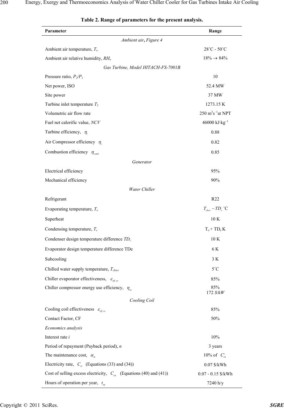

Energy, Exergy and Thermoeconomics Analysis of Water Chiller Cooler for Gas Turbines Intake Air Cooling 200
Table 2. Range of ptersarame for the present analysis.
Range Parameter
Ambient aFigure 4 ir,
Ambient air temperature, To 28˚C - 50˚C
Ambient air relative humidity, RHo 18% 84%
Gas Turbine, ModeTACH-FS-7001B
Pressure ratio, P2/P1 10
Net power, ISO 52.4 MW
Site power 37 MW
Turbine inlet temperature T3
Volumetric air flow rate
Fuel net calorific value, NCV
Turbine efficiency, t
l HI
1273.15 K
250 m3s–1at NPT
46000 kJ·kg–1

Air Compressor efficiency
0.88
c

0.82
Combustion efficiency 0.85
Generator
erature, Te
ature difference TDc 10
ference TDe
ate, Tchws 5
tiven s,
Chiller compressor energy use efficiency,
comb

Electrical efficiency
Mechanical efficiency
95%
90%
Water Chiller
Refrigerant R22
Evaporating tempchws e
TD˚C T
Superheat 10 K
Condensing temperature, Tc T
o + TDc K
Condenser design temperK
Evaporator design temperature dif6 K
Subcooling 3 K
Chilled water supply temperur˚C
Chiller evaporator effec es,effer  85%
eu

85%
172 $/kW
Cooling Coil
ss
Contact Factor, CF 50%
nalysis
10%
payment (Payback period), n 3
Cooling coil effectivene,effcc  85%
Economics a
Interest rate i
Period of reyears
The maintenance cost, m

10% of
c
ch
C
Electricity rate, el
C (Equations (33) and (34)) 0.07 $/kW
ns (40) and (41)) 0.07 - 0.15 $/kWh
ration per year, 7240 h/y
h
Cost of selling excess electricity, els C (Equatio
Hours of opeop t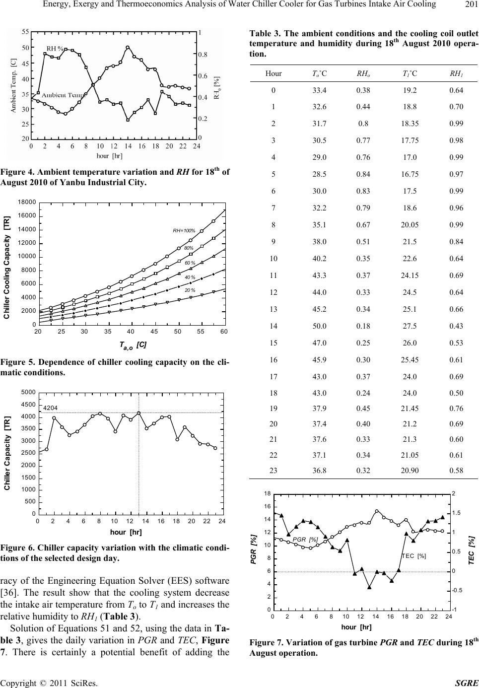

Energy, Exergy and Thermoeconomics Analysis of Water Chiller Cooler for Gas Turbines Intake Air Cooling201
Figure 4. Ambient tempth of
August 2010 of Yan
erature variation and RH for 18
bu Industrial City.
20253035 404550 55 60
0
2000
4000
6000
8000
10000
12000
14000
16000
18000
T
a
,
o
[C ]
Chiller Cooling Capacity [TR]
RH 100%
80%
60 %
40 %
20 %
Figure 5. Dependence of chiller cooling capacity on the cli-
matic conditions.
=
0 2 4 6 810 1214 16 18 20 22 24
0
500
1000
1500
2000
2500
3000
3500
4000
4500
5000
hour [hr]
Chiller Capacity [TR]
4204
Figure 6. Chiller capacity variation with the climatic condi-
tions of the selected design day.
show that the cooling system decrease
e intake air temperature from To to T1 and increases the
relative humidity to RH1 (Table 3).
Solution of Equations 51 and 52, using the data in Ta-
ble 3, gives the daily variation in PGR and TEC, Figure
7. There is certainly a potential benefit of adding the
Table 3. The ambient cond and the cooling coil outlet
temperature and humidity durth August 2010 opera-
tion.
Hour To˚C T1˚C RH1
racy of the Engineering Equation Solver (EES) software
36]. The result [
th
itions
ing 18
RHo
0 33.4 0.38 19.2 0.64
1 32.6 18.8 0.70
2 31.7 18.35 0.99
3 30.5 0.77 17.75 0.98
4 29.0 17.0 0.99
5 28.5 16.75 0.97
6 30.0 17.5 0.99
32.2 18.6 0.96
8 35.1 20.05 0.99
9 38.0 0.51 21.5 0.84
10 40.2 0.35 22.6 0.64
11 43.3 0.37 24.15 0.69
12 44.0 0.33 24.5 0.64
13 45.2 0.34 25.1 0.66
14 50.0 0.18 27.5 0.43
15 47.0 0.25 26.0 0.53
16 45.9 0.30 25.45 0.61
17 43.0 0.37 24.0 0.69
18 43.0 0.24 24.0 0.50
20 37.4 0.40 21.2 0.69
20.90 0.58
0.44
0.8
0.76
0.84
0.83
7 0.79
0.67
19 37.9 0.45 21.45 0.76
21 37.6 0.33 21.3 0.60
22 37.1 0.34 21.05 0.61
23 36.8 0.32
0246810 1214 16 18 20 22 24
0
2
4
6
8
10
12
14
16
18
-1
-0.5
0
0.5
1
1.5
2
hou
PG R TEC [%]
PGR [%]
]
Figur. Variat gas tuPGR EC during 18th
August operation.
r [hr]
[%]
TEC [%
e 7ion ofrbine and T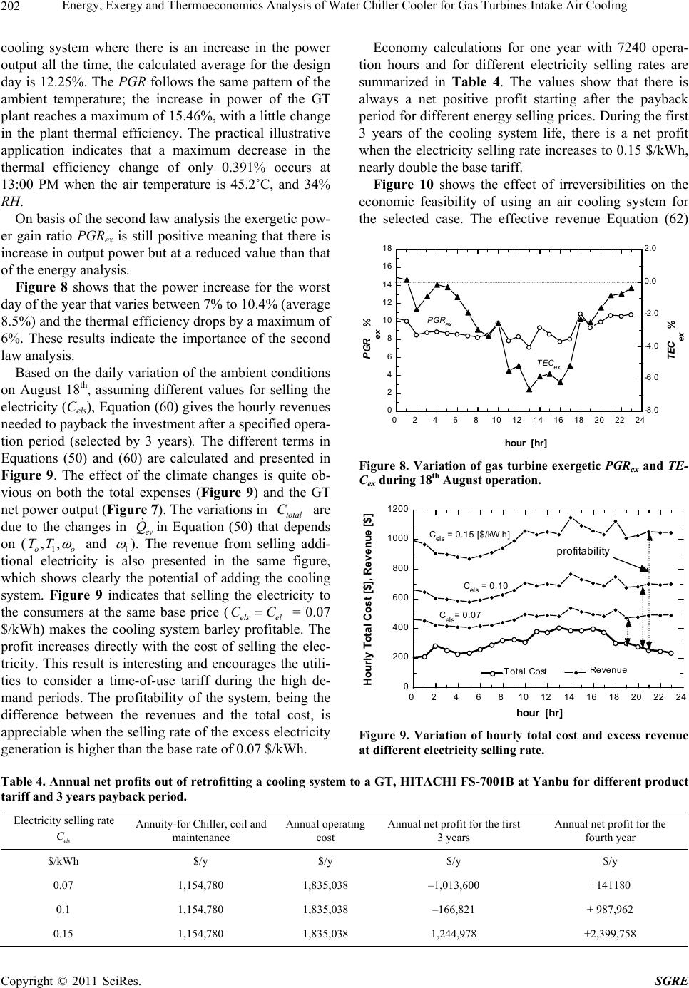

Energy, Exergy and Thermoeconomics Analysis of Water Chiller Cooler for Gas Turbines Intake Air Cooling 202
cooling systemre the the power
output all the tihe design
day is 12.25%.PGR e pattern of the
ambient temperature; the ner of
plant reaches a mum .46%,lege
in the plant therme pe
appliion inds thataximucreasehe
thermefficiechangonly 0.391% ocat
13:00 PM when the air temperature is 45.2˚C, and 34%
RH.
On basis of tcond lnalysisxergetw-
er ga PGR is still itive meang that th
increase in output a reduced value than that
of the energy analysis.
Figure 8 shohat thincrease for the worst
day of the year that varies between 7% to 10.4% (average
8.5%d the tal effiy drop maxi of
6%. se resucateimportof the second
law analysis.
Ba on the variof the ent cons
on Ast 18th ming rent vor selhe
electricity (Cels)ation ves turly res
needo paybnvnt afteecifiedra-
tion peod (sel 3 y. The t term
Equas (50)60) alculat prese in
Figure 9. The effect of thmate changes is quite ob-
ious on both the total expenses (Figure 9) and the GT
net power output (Figure 7). The variations in are
due to the changes in n Equation (50) thnds
on (
where is an increase in
me, the calculated ave
The
rage for t
samefollows th
increase i powthe GT
maxi
al efficien
of 15
cy. Th
with a litt
ractical illu
chan
strativ
caticate a mm de in t
al ncy e of curs
he seaw a the eic po
in ratioex
power but
pos
at
inere is
ws te power
) anhermciencs by amum
Thelts indi the ance
sed dailyation ambinditio
ugu, assudiffealues fling t
, Equ(60) gihe hoevenu
ed t
ri
ack the i
ected by
estme
ears)
r a sp
differen
ope
s in
tion and (re caed andnted
e cli
v
total
C
at depe
ev
Q
i
1
,,
oo
TT

and 1

). Th
e po
e
ing
e revenue from sel-
tional electricity is also presented in the sam figure,
wh shows clearly thtential of adding thling
syste indicates that selling the
ers at the sam base price (0.07
$/khsystem barl The
profit increases directly with the cost of selling the elec-
tricity. This result is interesting and encourages the utili-
ties to consider a time-of-use tariff during the high de-
mand periods. The profitability of the system, being th
. The values show that there is
al
the base tariff.
ling addi
e
e coo
electricity to
el =
table.
ich
m. Figure 9
the consum
Wh) makes t
els
CC
ey profie cool
e
difference between the revenues and the total cost, is
appreciable when the selling rate of the excess electricity
generation is higher than the base rate of 0.07 $/kWh.
Economy calculations for one year with 7240 opera-
tion hours and for different electricity selling rates are
summarized in Table 4
ways a net positive profit starting after the payback
period for different energy selling prices. During the first
3 years of the cooling system life, there is a net profit
when the electricity selling rate increases to 0.15 $/kWh,
nearly double
Figure 10 shows the effect of irreversibilities on the
economic feasibility of using an air cooling system for
the selected case. The effective revenue Equation (62)
0 2 4 6 810 121416 18
6
0
2
4
20 2224
8
10
12
14
16
18
-8.0
-6.0
-4.0
-2.0
0.0
2.0
h our [hr]
PGR
ex
%
TEC
ex
%
TECex
PGRex
Figure 8. Variation of gas turbine exergetic PGRex and TE-
Cex during 18th August operation.
0246810 1214 16 182022 2
4
0
200
400
600
800
1000
1200
hou
Hourly To tal Cost
C
el s
= 0.0 7
C
el s
= 0.10
Revenue
r [hr ]
[$], Revenu e [$]
C
el s
= 0.15 [$/kW h]
Total Cost
profitability
Fi
to aT, HITACHI FS-7001B at Yanbu for different product
rating Annual net profit for the first
3 years
Annual net profit for the
fourth year
gure 9. Variation of hourly total cost and excess revenue
at different electri ci ty selling rate.
Table 4. Annual net profits out of retrofitting a cooling system
tariff and 3 years pay bac k period.
Electricity selling rate
els
C
Annuity-for Chiller, coil and
maintenance
Annual ope
cost
G
$/kWh $/y $/y $/y $/y
0.07 1,154,780 1,835,038 –1,013,600 +141180
0.1 1,154,780 1,835,038 –166,821 + 987,962
38 1,244,978 +2,399,758 0.15 1,154,780 1,835,0
C
opyright © 2011 SciRes. SGRE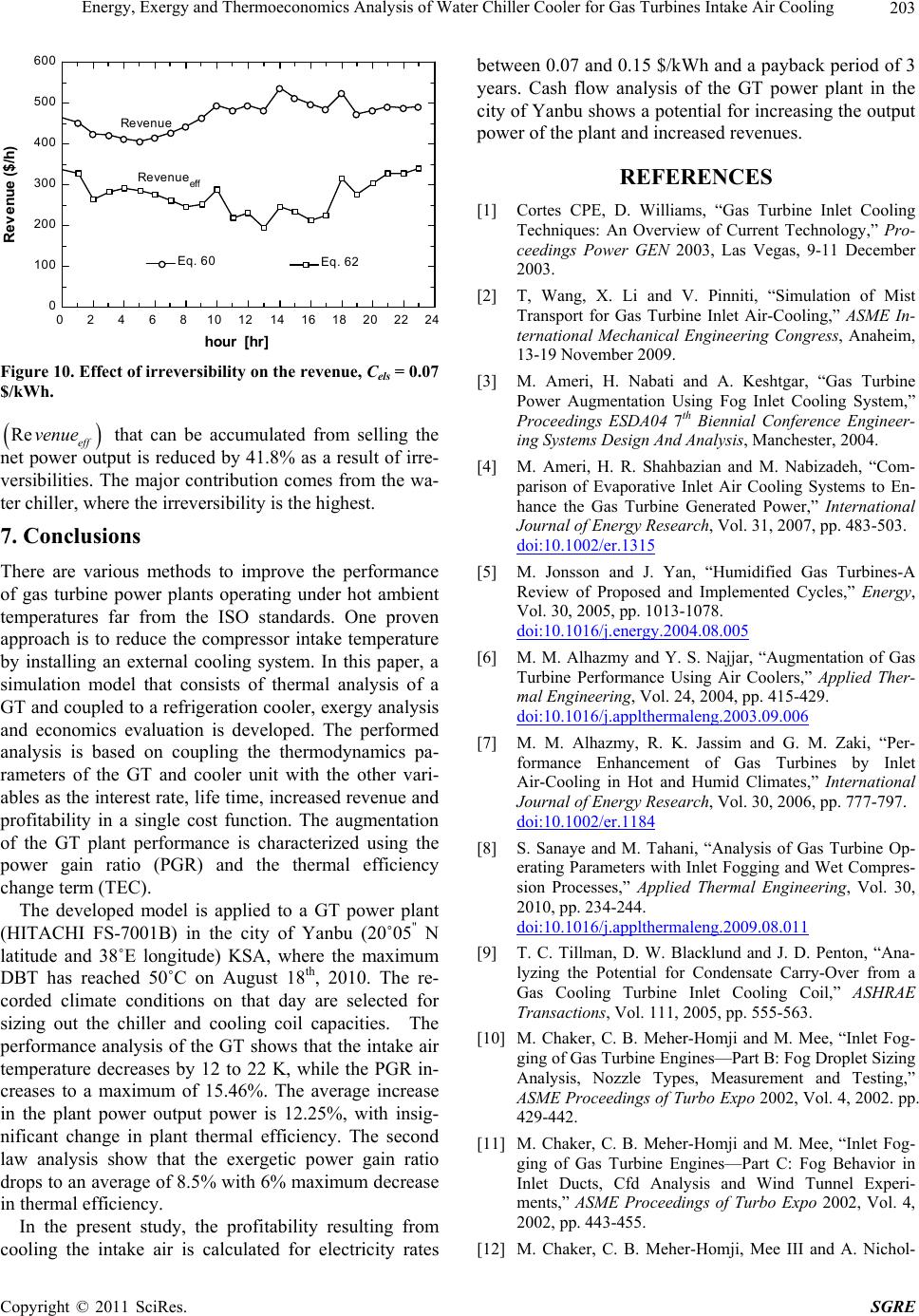

Energy, Exergy and Thermoeconomics Analysis of Water Chiller Cooler for Gas Turbines Intake Air Cooling203
0 2 4 6 810 1214 16182022 2
4
0
100
200
300
400
500
600
Revenue ($/h)
Revenue
Revenue
eff
hour [hr]
Eq. 62Eq. 62
Eq. 60Eq. 60
Figure 10. Effect of irreversibility on the revenue, Cels = 0.07
ulated from selling the
ed l
versibilities. The major contres from the w
ter chille irreversibility is the highest.
7. Conclusions
There arerious methods to the perform
of gas turbine power plants operating under hot ambient
mperatures far from the ISO standards. One pr
pproach is to reduce the compressor intake temperature
by installing an external cooling system. In this paper, a
simulation model that consists of thermal analysis of a
GT and coupled to a refrigeration cooler, exergy analysis
and economics evaluation is developed. The performed
analysis is based on coupling the thermodynamics pa-
rameters of the GT and cooler unit with the other vari-
ables as the interest rate, life time, increased revenue and
profitability in a single cost function. The augmentation
of the GT plant performance is characterized using the
power gain ratio (PGR) and the thermal efficiency
change term (TEC).
The developed model is applied to a GT power plant
(HITACHI FS-7001B) in the city of Yanbu (20˚05" N
s reached 50˚C on August 18, 2010. The re-
d climate conditions on that day are selected for
sizing out th
rease
output power is 12.25%, with insig-
plant thermal efficiency. The second
between 0.07 and 0.15 $/kWh and a payback period of 3
years. Cash flow analysis of the GT power plant in the
city of Yanbu shows a potential for increasing the output
power of the plant and increased revenues.
REFERENCES
[1] Cortes CPE, D. Williams, “Gas Turbine Inlet Cooling
Techniques: An Overview of Current Technology,” Pro-
ceedings Power GEN 2003, Las Vegas, 9-11 December
2003.
[2] T, Wang, X. Li and V. Pinniti, “Simulation of Mist
Transport for Gas Turbine Inlet Air-Cooling,” ASME In-
ternational Mechanical Engineering Congress, Anaheim
Keshtgar, “Gas Turbine
ing Systems Design And Analysis, Manchester, 2004.
ian a-
parison oe Inlet Air Coos to En-
hance the Gas Turbine Generated Poweternational
Journal of En, Vol. 31, 2007. 483-503.
doi:10. 5
$/kWh.

Re eff venue that can be accum
Power Augmentation Using Fog Inlet Cooling System,”
Proceedings ESDA04 7th Biennial Conference Engineer-
net power output is ruced by 41.8% as a resu
ibution com
t of irre-
a- [4]
er, where th
va improveance
te
a
oven
latitude and 38˚E longitude) KSA, where the maximum
DBT hath
corde
e chiller and cooling coil capacities. The
performance analysis of the GT shows that the intake air
temperature decreases by 12 to 22 K, while the PGR in-
creases to a maximum of 15.46%. The average inc
in the plant power
nificant change in
law analysis show that the exergetic power gain ratio
drops to an average of 8.5% with 6% maximum decrease
in thermal efficiency.
In the present study, the profitability resulting from
cooling the intake air is calculated for electricity rates
,
13-19 November 2009.
[3] M. Ameri, H. Nabati and A.
M. Ameri, H. R. Shahbaz
f Evaporativ
nd M. Nabizadeh, “Com
ling System
r,” In
, ppergy Research
1002/er.131
[5] M. Jonsson and J. Yan, “Humidifirbines-A
Review of Implemented CEnergy,
Vol. 30.
doi:10.1016/j.energy.2004.08.005
ed Gas Tu
ycles,” Proposed and
, 2005, pp. 1013-1078
[6] M. M. Alhazmy and Y. S. Najjar, “Augmentation of Gas
Turbine Performance Using Air Coolers,” Applied Ther-
mal Engineering, Vol. 24, 2004, pp. 415-429.
doi:10.1016/j.applthermaleng.2003.09.006
[7] M. M. Alhazmy, R. K. Jassim and G. M. Zaki, “Per-
formance Enhancement of Gas Turbines by Inlet
Air-Cooling in Hot and Humid Climates,” International
Journal of Energy Research, Vol. 30, 2006, pp. 777-797.
doi:10.1002/er.1184
[8] S. Sanaye and M. Tahani, “Analysis of Gas Turbine Op-
erating Parameters with Inlet Fogging and Wet Compres-
sion Processes,” Applied Thermal Engineering, Vol. 30,
2010, pp. 234-244.
doi:10.1016/j.applthermaleng.2009.08.011
[9] T. C. Tillman, D. W. Blacklund and J. D. Penton, “Ana-
lyzing the Potential for Condensate Carry-Over from a
Gas Cooling Turbine Inlet Cooling Coil,” ASHRAE
Transactions, Vol. 111, 2005, pp. 555-563.
[10] M. Chaker, C. B. Meher-Homji and M. Mee, “Inlet Fog-
ging of Gas Turbine Engines—Part B: Fog Droplet Sizing
Analysis, Nozzle Types, Measurement and Testing,”
ASME Proceedings of Turbo Expo 2002, Vol. 4, 2002. pp.
429-442.
[11] M. Chaker, C. B. Meher-Homji and M. Mee, “Inlet Fog-
ging of Gas Turbine Engines—Part C: Fog Behavior in
Inlet Ducts, Cfd Analysis and Wind Tunnel Experi-
ments,” ASME Proceedings of Turbo Expo 2002, Vol. 4,
2002, pp. 443-455.
[12] M. Chaker, C. B. Meher-Homji, Mee III and A. Nichol-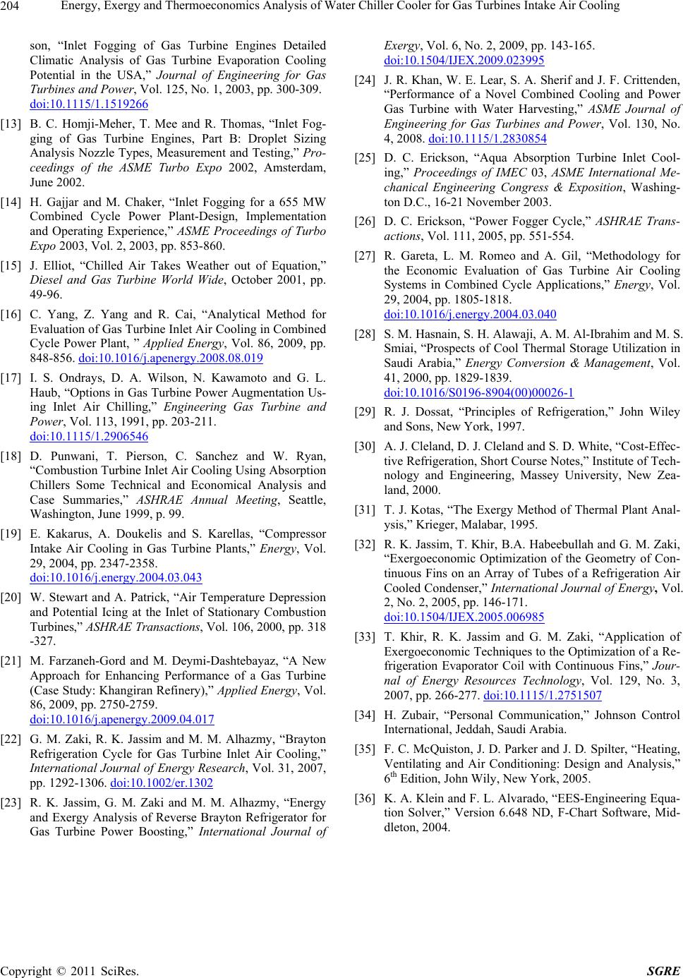

Energy, Exergy and Thermoeconomics Analysis of Water Chiller Cooler for Gas Turbines Intake Air Cooling 204
son, “Inlet Fogging of Gas Turbine Engines Detailed
Climatic Analysis of Gas Turbine Evaporation Cooling
Potential in the USA,” Journal of Engineering for Gas
Turbines and Power, Vol. 125, No. 1, 2003, pp. 300-309.
doi:10.1115/1. 1519266
eher, T. Mee and R. T[13] B. C. Homji-Mhomas, “Inlet Fog-
02.
pp. 853-860.
for
ging of Gas Turbine Engines, Part B: Droplet Sizing
Analysis Nozzle Types, Measurement and Testing,” Pro-
ceedings of the ASME Turbo Expo 2002, Amsterdam,
June 20
[14] H. Gajjar and M. Chaker, “Inlet Fogging for a 655 MW
Combined Cycle Power Plant-Design, Implementation
and Operating Experience,” ASME Proceedings of Turbo
Expo 2003, Vol. 2, 2003,
[15] J. Elliot, “Chilled Air Takes Weather out of Equation,”
Diesel and Gas Turbine World Wide, October 2001, pp.
49-96.
[16] C. Yang, Z. Yang and R. Cai, “Analytical Method
Evaluation of Gas Turbine Inlet Air Cooling in Combined
Cycle Power Plant, ” Applied Energy, Vol. 86, 2009, pp.
848-856. doi:10.1016/j.apenergy.2008.08.019
[17] I. S. Ondrays, D. A. Wilson, N. Kawamoto and G. L.
Haub, “Options in Gas Turbine Power Augmentation Us-
ing Inlet Air Chilling,” Engineering Gas Turbine and
Power, Vol. 113, 1991, pp. 203-211.
doi:10.1115/1.2906546
[18] D. Punwani, T. Pierson, C. Sanchez and W. Ryan,
, Seattle,
“Combustion Turbine Inlet Air Cooling Using Absorption
Chillers Some Technical and Economical Analysis and
Case Summaries,” ASHRAE Annual Meeting
Washington, June 1999, p. 99.
[19] E. Kakarus, A. Doukelis and S. Karellas, “Compressor
Intake Air Cooling in Gas Turbine Plants,” Energy, Vol.
29, 2004, pp. 2347-2358.
doi:10.1016/j.energy.2004.03.043
[20] W. Stewart and A. Patrick, “Air Temperature Depression
yaz, “A New
and Potential Icing at the Inlet of Stationary Combustion
Turbines,” ASHRAE Transactions, Vol. 106, 2000, pp. 318
-327.
[21] M. Farzaneh-Gord and M. Deymi-Dashteba
Approach for Enhancing Performance of a Gas Turbine
(Case Study: Khangiran Refinery),” Applied Energy, Vol.
86, 2009, pp. 2750-2759.
doi:10.1016/j.apenergy.2009.04.017
[22] G. M. Zaki, R. K. Jassim and M. M. Alhazmy, “Brayton
Refrigeration Cycle for Gas Turbine Inlet Air Cooling,”
International Journal of Energy Research, Vol. 31, 2007,
pp. 1292-1306. doi:10.1002/er.1302
[23] R. K. Jassim, G. M. Zaki and M. M. Alhazmy, “Energy
and Exergy Analysis of Reverse Brayton Refrigerator for
Gas Turbine Power Boosting,” International Journal of
Exergy, Vol. 6, No. 2, 2009, pp. 143-165.
doi:10.1504/IJEX.2009.023995
[24] J. R. Khan, W. E. Lear, S. A. Sherif and J. F. Crittenden,
“Performance of a Novel Combined Cooling and Power
Gas Turbine with Water Harvesting,” ASME Journal of
Engineering for Gas Turbines and Power, Vol. 130, No.
4, 2008. doi:10.1115/1.2830854
[25] D. C. Erickson, “Aqua Absorption Turbine Inlet Cool-
ing,” Proceedings of IMEC 03, ASME International Me-
n Combined Cycle Applications,” Energy, Vol.
chanical Engineering Congress & Exposition, Washing-
ton D.C., 16-21 November 2003.
[26] D. C. Erickson, “Power Fogger Cycle,” ASHRAE Trans-
actions, Vol. 111, 2005, pp. 551-554.
[27] R. Gareta, L. M. Romeo and A. Gil, “Methodology for
the Economic Evaluation of Gas Turbine Air Cooling
Systems i
29, 2004, pp. 1805-1818.
doi:10.1016/j.energy.2004.03.040
[28] S. M. Hasnain, S. H. Alawaji, A. M. Al-Ibrahim and M. S.
Smiai, “Prospects of Cool Thermal Storage Utilization in
Saudi Arabia,” Energy Conversion & Management, Vol.
41, 2000, pp. 1829-1839.
doi:10.1016/S0196-8904(00)00026-1
[29] R. J. Dossat, “Principles of Refrigera
and Sons, New York, 19
tion,” John Wiley
97.
the Geometry of Con-
[30] A. J. Cleland, D. J. Cleland and S. D. White, “Cost-Effec-
tive Refrigeration, Short Course Notes,” Institute of Tech-
nology and Engineering, Massey University, New Zea-
land, 2000.
[31] T. J. Kotas, “The Exergy Method of Thermal Plant Anal-
ysis,” Krieger, Malabar, 1995.
[32] R. K. Jassim, T. Khir, B.A. Habeebullah and G. M. Zaki,
“Exergoeconomic Optimization of
tinuous Fins on an Array of Tubes of a Refrigeration Air
Cooled Condenser,” International Journal of Energy, Vol.
2, No. 2, 2005, pp. 146-171.
doi:10.1504/IJEX.2005.006985
[33] T. Khir, R. K. Jassim and G. M. Zaki, “Application of
Exergoeconomic Techniques to the Optimization of a Re-
frigeration Evaporator Coil with Continuous Fins,” Jour-
nal of Energy Resources Technology, Vol. 129, No. 3,
2007, pp. 266-277. doi:10.1115/1.2751507
[34] H. Zubair, “Personal Communication,” Johnson Control
International, Jeddah, Saudi Arabia.
[35] F. C. McQuiston, J. D. Parker and J. D. Spilter, “Heating,
Ventilating and Air Conditioning: Design and Analysis,”
th
6 Edition, John Wily, New York, 2005.
[36] K. A. Klein and F. L. Alvarado, “EES-Engineering Equa-
tion Solver,” Version 6.648 ND, F-Chart Software, Mid-
dleton, 2004.
C
opyright © 2011 SciRes. SGRE

Energy, Exergy and Thermoeconomics Analysis of Water Chiller Cooler for Gas Turbines Intake Air Cooling205
Nomenclatures
Acc Cooling coil heat transfer area, m2
c
cc
C capital cost of cooling coil ($)
c
ch
C capital cost of chiller ($)
el
C unit cost of electricity, $/kWh
p
c specific heat of gases, kJ/kg K
CF contact factor
E energy kWh
EES engineering Equation Solver
hv specific enthalpy of water vapor in the air, kJ/kg
i interest rate on capital
I
 exergy destruction, kW
k specific heats ratio.
m
 mass flow rate, kg s–1
m
 air mass flow rate, kg/s
a
cw
m
 chilled water mass flow rate, kg/s
r
m  refrigerant mass flow rate, kg/s
condensate
w
m
 water rate, kg/s
NCV net calorific value, kJ kg–1
P pressure, kPa
PGR power gain ratio
Po atmospheric pressure, kPa
PR pressure ratio = P2/P1
heat rate, kW
chiller evaporator cooling capacity, kW
cooling coil thermal capacity, kW
h
Q

,er
Q

cc
Q

S
 entropy, kJ/K
t time, s
T Temperature, K
TEC thermal efficiency change factor
U overall heat transfer coefficient, kW/m2K
x quality.
W
 power, Kw
Greek Symbols

efficiency
eff

effectiveness, according to subscripts

specific humidity (also, humidity ratio), according
to subscripts, kg/kgdry air
Subscripts
dry air a
c with cooling
cc cooling coil
ch chiller
comb combustion
comp compressor
eff effective
el electricity
f fuel
g gas
nc no cooling
o ambient
t turbine
v vapor
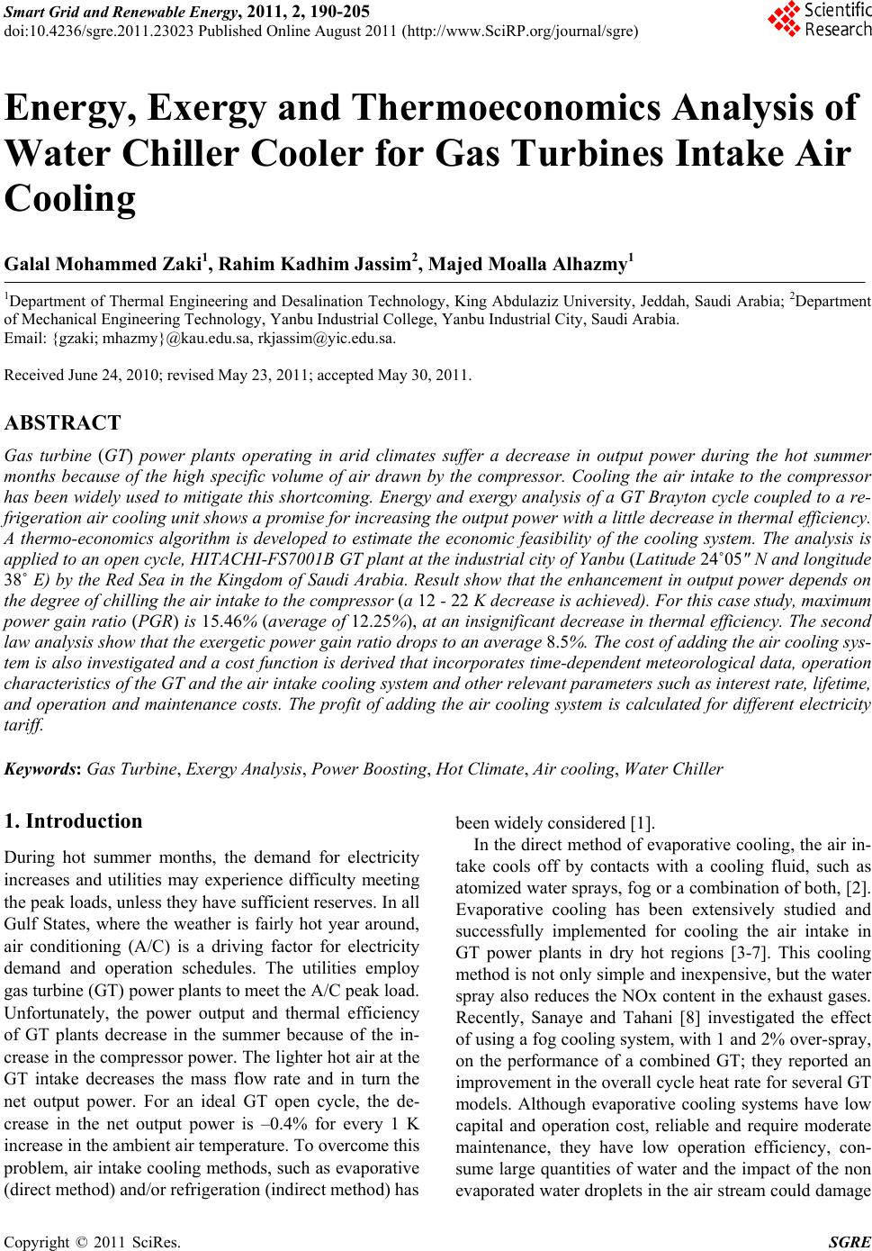