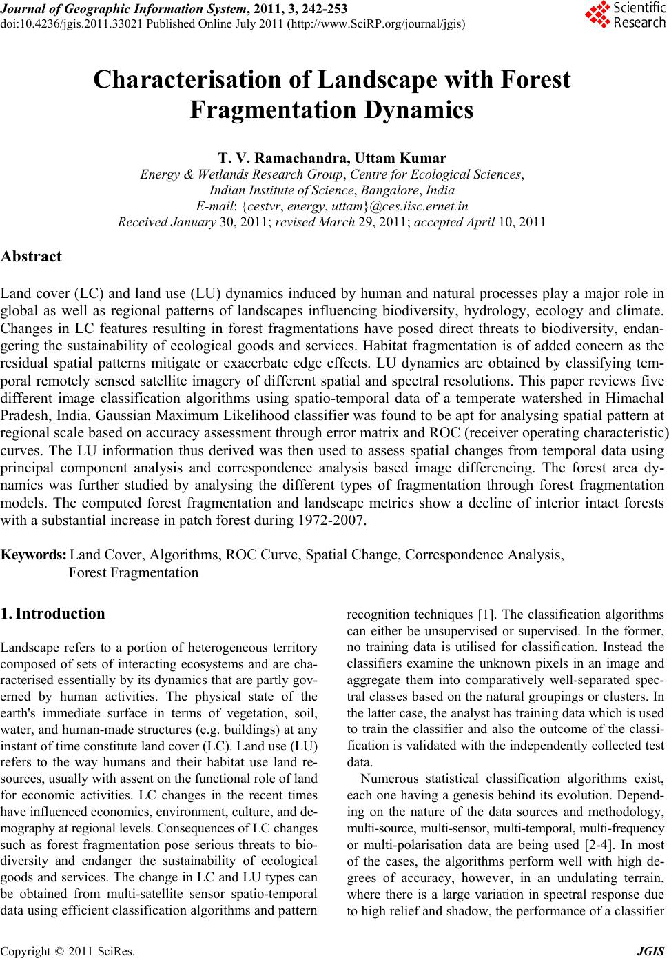Journal of Geographic Information System, 2011, 3, 242-253
doi:10.4236/jgis.2011.33021 Published Online July 2011 (http://www.SciRP.org/journal/jgis)
Characterisation of Landscape with Forest
Fragmentation Dynamics
T. V. Ramachandra, Uttam Kumar
Energy & Wetlands Research Group, Centre for Ecological Sciences,
Indian Institute of Science, Bangalore, India
Received January 30, 2011; revised March 29 , 20 1 1; accepted April 10 , 2011
Abstract
Land cover (LC) and land use (LU) dynamics induced by human and natural processes play a major role in
global as well as regional patterns of landscapes influencing biodiversity, hydrology, ecology and climate.
Changes in LC features resulting in forest fragmentations have posed direct threats to biodiversity, endan-
gering the sustainability of ecological goods and services. Habitat fragmentation is of added concern as the
residual spatial patterns mitigate or exacerbate edge effects. LU dynamics are obtained by classifying tem-
poral remotely sensed satellite imagery of different spatial and spectral resolutions. This paper reviews five
different image classification algorithms using spatio-temporal data of a temperate watershed in Himachal
Pradesh, India. Gaussian Maximum Likelihood classifier was found to be apt for analysing spatial pattern at
regional scale based on accuracy assessment through erro r matrix and ROC (receiver operating characteristic)
curves. The LU information thus derived was then used to assess spatial changes from temporal data using
principal component analysis and correspondence analysis based image differencing. The forest area dy-
namics was further studied by analysing the different types of fragmentation through forest fragmentation
models. The computed forest fragmentation and landscape metrics show a decline of interior intact forests
with a substantial increase in patch forest during 1972-2007.
Keywords: Land Cover, Algorithms, ROC Curve, Spatial Change, Correspondence Analysis,
Forest Fragmentation
1. Introduction
Landscape refers to a portion of heterogeneous territory
composed of sets of interacting ecosystems and are cha-
racterised essentially by its dynamics that are partly gov-
erned by human activities. The physical state of the
earth's immediate surface in terms of vegetation, soil,
water, and human-made structures (e.g. buildings) at any
instant of time constitu te land co ver (LC). Land us e (LU)
refers to the way humans and their habitat use land re-
sources, usually with assent on the functional role of land
for economic activities. LC changes in the recent times
have influenced economics, environment, culture, and de-
mography at regional levels. Consequences of LC changes
such as forest fragmentation pose serious threats to bio-
diversity and endanger the sustainability of ecological
goods and services. The change in LC and LU types can
be obtained from multi-satellite sensor spatio-temporal
data using efficient classification algorithms and pattern
recognition techniques [1]. The classification algorithms
can either be unsupervised or supervised. In the former,
no training data is utilised for classification. Instead the
classifiers examine the unknown pixels in an image and
aggregate them into comparatively well-separated spec-
tral classes based on the natural groupings or clusters. In
the latter case, the analyst has training data which is used
to train the classifier and also the outcome of the classi-
fication is validated with the independently collected test
data.
Numerous statistical classification algorithms exist,
each one having a genesis behind its evolution. Depend-
ing on the nature of the data sources and methodology,
multi-source, multi-sensor, multi-temporal, multi-frequency
or multi-polarisation data are being used [2-4]. In most
of the cases, the algorithms perform well with high de-
grees of accuracy, however, in an undulating terrain,
where there is a large variation in spectral response due
to high relief and shadow, the performance of a classifier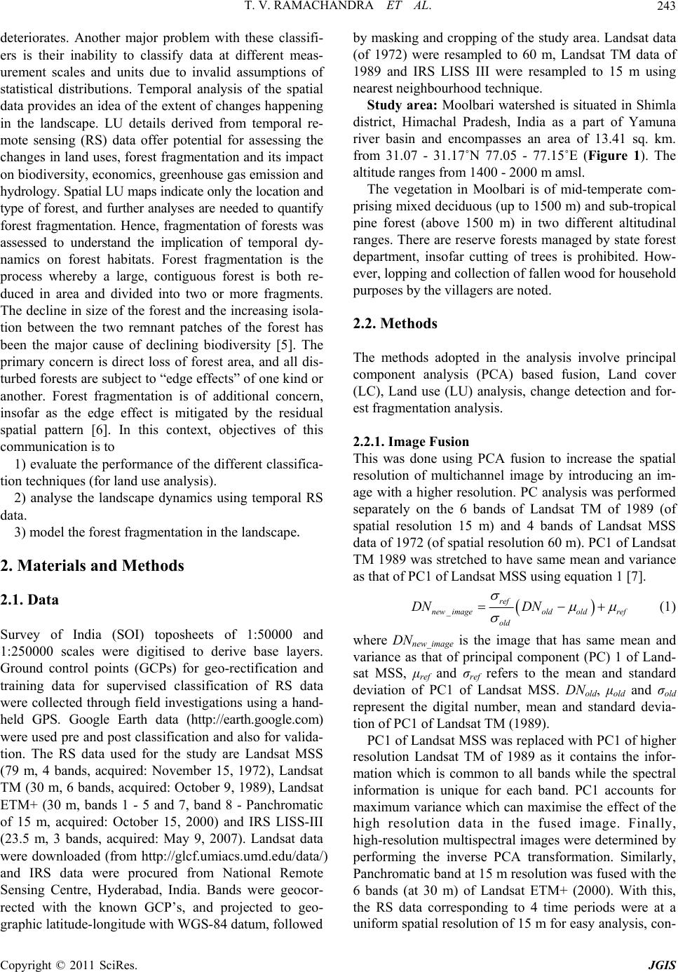

T. V. RAMACHANDRA ET AL. 243
deteriorates. Another major problem with these classifi-
ers is their inability to classify data at different meas-
urement scales and units due to invalid assumptions of
statistical distributions. Temporal analysis of the spatial
data provides an idea of the extent of ch anges happening
in the landscape. LU details derived from temporal re-
mote sensing (RS) data offer potential for assessing the
changes in land uses, forest fragmentation and its impact
on biodiversity, economics, greenhouse gas emission and
hydrology. Spatial LU maps indicate only the location and
type of forest, and further analyses are needed to quantify
forest fragmentation. Hence, fragmentation of forests was
assessed to understand the implication of temporal dy-
namics on forest habitats. Forest fragmentation is the
process whereby a large, contiguous forest is both re-
duced in area and divided into two or more fragments.
The decline in size of the forest and the increasing isola-
tion between the two remnant patches of the forest has
been the major cause of declining biodiversity [5]. The
primary concern is direct loss of forest area, and all dis-
turbed forests are subject to “edge effects” of one kind or
another. Forest fragmentation is of additional concern,
insofar as the edge effect is mitigated by the residual
spatial pattern [6]. In this context, objectives of this
communication is to
1) evaluate the performance of the different classifica-
tion techniques (for land use analysis).
2) analyse the landscape dynamics using temporal RS
data.
3) model the forest fragmentation in the landscape.
2. Materials and Methods
2.1. Data
Survey of India (SOI) toposheets of 1:50000 and
1:250000 scales were digitised to derive base layers.
Ground control points (GCPs) for geo-rectification and
training data for supervised classification of RS data
were collected through field investigations using a hand-
held GPS. Google Earth data (http://earth.google.com)
were used pre and post classification and also for valida-
tion. The RS data used for the study are Landsat MSS
(79 m, 4 bands, acquired: November 15, 1972), Landsat
TM (30 m, 6 bands, acquired: October 9, 1989), Landsat
ETM+ (30 m, bands 1 - 5 and 7, band 8 - Panchromatic
of 15 m, acquired: October 15, 2000) and IRS LISS-III
(23.5 m, 3 bands, acquired: May 9, 2007). Landsat data
were downloaded (from http://glcf.umiacs.umd.edu/data/)
and IRS data were procured from National Remote
Sensing Centre, Hyderabad, India. Bands were geocor-
rected with the known GCP’s, and projected to geo-
graphic latitude-longitude with WGS-84 datum, followed
by masking and cropping of the study area. Landsat data
(of 1972) were resampled to 60 m, Landsat TM data of
1989 and IRS LISS III were resampled to 15 m using
nearest neighbourhood technique.
Study area: Moolbari watershed is situated in Shimla
district, Himachal Pradesh, India as a part of Yamuna
river basin and encompasses an area of 13.41 sq. km.
from 31.07 - 31.17˚N 77.05 - 77.15˚E (Figure 1). The
altitude ranges from 1400 - 2000 m amsl.
The vegetation in Moolbari is of mid-temperate com-
prising mixed deciduous (up to 1500 m) and sub-tropical
pine forest (above 1500 m) in two different altitudinal
ranges. There are reserve forests managed by state forest
department, insofar cutting of trees is prohibited. How-
ever, lopping and collection of fallen wood for household
purposes by the villagers are noted.
2.2. Methods
The methods adopted in the analysis involve principal
component analysis (PCA) based fusion, Land cover
(LC), Land use (LU) analysis, change detection and for-
est fragmentation analysis.
2.2.1. Image Fusion
This was done using PCA fusion to increase the spatial
resolution of multichannel image by introducing an im-
age with a higher resolution. PC analysis was performed
separately on the 6 bands of Landsat TM of 1989 (of
spatial resolution 15 m) and 4 bands of Landsat MSS
data of 1972 (of spatial resolution 60 m). PC1 of Landsat
TM 1989 was stretched to have same mean and variance
as that of PC1 of Landsat MSS using equation 1 [7].

_
ref
new imageoldoldref
old
DN DN




 (1)
where DNnew_image is the image that has same mean and
variance as that of principal component (PC) 1 of Land-
sat MSS, μref and σref refers to the mean and standard
deviation of PC1 of Landsat MSS. DNold, μold and σold
represent the digital number, mean and standard devia-
tion of PC1 of Landsat TM (1989).
PC1 of Landsat MSS was replaced with PC1 of higher
resolution Landsat TM of 1989 as it contains the infor-
mation which is common to all bands while the spectral
information is unique for each band. PC1 accounts for
maximum variance which can maximise the effect of the
high resolution data in the fused image. Finally,
high-resolution multispectral imag es were determined by
performing the inverse PCA transformation. Similarly,
Panchromatic band at 15 m resolution was fused with the
6 bands (at 30 m) of Landsat ETM+ (2000). With this,
the RS data corresponding to 4 time periods were at a
uniform spatial resolution of 15 m for easy analysis, con-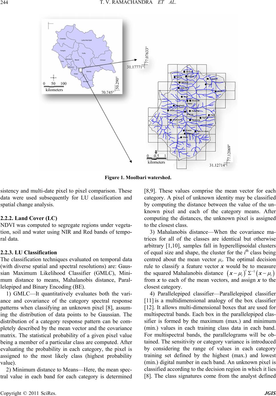

T. V. RAMACHANDRA ET AL. 244
Figure 1. Moolbari watershed.
sistency and multi-date pixel to pixel comparison. These
data were used subsequently for LU classification and
spatial change analysis.
2.2.2. Land Cover (LC)
NDVI was computed to segregate regions under vegeta-
tion, soil and water using NIR and Red bands of tempo-
ral data.
2.2.3. LU Classification
The classification techniques evaluated on temporal data
(with diverse spatial and spectral resolutions) are: Gaus-
sian Maximum Likelihood Classifier (GMLC), Mini-
mum distance to means, Mahalanobis distance, Paral-
lelepiped and Binary Encoding (BE).
1) GMLC—It quantitatively evaluates both the vari-
ance and covariance of the category spectral response
patterns when classifying an unknown pixel [8], assum-
ing the distribution of data points to be Gaussian. The
distribution of a category response pattern can be com-
pletely described by the mean vector and the covariance
matrix. The statistical probability of a given pixel value
being a member of a particular class are computed. After
evaluating the probability in each category, the pixel is
assigned to the most likely class (highest probability
value).
2) Min imum distance to Means—Here, the mean spec-
tral value in each band for each category is determined
[8,9]. These values comprise the mean vector for each
category. A pixel of unknown identity may be classified
by computing the distance between the value of the un-
known pixel and each of the category means. After
computing the distances, the unknown pixel is assigned
to the closest class.
3) Mahalanobis distance—When the covariance ma-
trices for all of the classes are identical but otherwise
arbitrary [1,10], samples fall in hyperellipsoidal clusters
of equal size and shape, the cluster for the ith class being
centred about the mean vector μi. The optimal decision
rule to classify a feature vector x would be to measure
the squared Mahalanobis distance

1
t
ii


 xx
from x to each of the mean vectors, and assign x to the
closest category.
4) Parallelepiped classifier—Parallelepiped classifier
[11] is a multidimensional analogy of the box classifier
[12]. It allows multi-dimensional boxes that are used for
multispectral bands. Each box in the parallelepiped clas-
sifier is formed by the maximum (max.) and minimum
(min.) values in each training class data in each band.
For multispectral bands, the parallelograms will be ob-
tained. The sensitivity or category varian ce is introduced
by considering the range of values in each category
training set defined by the highest (max.) and lowest
(min.) digital number in each band. An unknown pixel is
classified according to the decision region in which it lies
[8]. The class signatures come from the analyst defined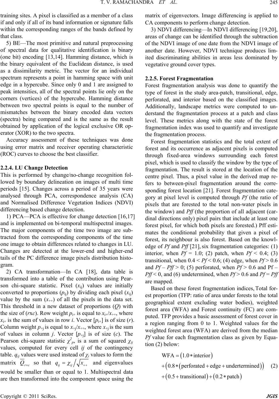

T. V. RAMACHANDRA ET AL. 245
training sites. A pixel is classified as a member of a class
if and only if all of its band information or signature falls
within the corresponding ranges of the bands defined by
that class.
5) BE—The most primitive and natural preprocessing
of spectral data for qualitative identification is binary
(one bit) encoding [13,14]. Hamming distance, which is
the binary equivalent of the Euclidean distance, is used
as a dissimilarity metric. The vector for an individual
spectrum represents a point in hamming space with unit
edge in a hypercube. Since only 0 and 1 are assigned to
peak intensities, all of the spectral points lie only on the
corners (vertices) of the hypercube. Hamming distance
between two spectral points is equal to the number of
mismatches between the binary encoded data vectors
(spectra) being compared and is the same as the result
obtained by application of the logical exclusive OR op-
erator (XOR) to the two spectra.
Accuracy assessment of these techniques was done
using error matrix and receiver operating characteristic
(ROC) curves to choose the best classifier.
2.2.4. LU Change Detection
This is performed by change/no-change recognition fol-
lowed by boundary delineation on images of multi time
periods [15]. Changes across a period of 35 years were
analysed through PCA, correspondence analysis (CA)
and Normalised Difference Vegetation Indices (NDVI)
differencing based change detection.
1) PCA—PCA is effective for change detection [16,17]
and is implemented on bi-temporal multispectral images.
The major components of the time two image are sub-
tracted from the corresponding components of the time
one image to obtain differences related to changes in LU.
Changes are detected at the lower-end and higher-end
tails of the PC difference image pixels distribution histo-
gram.
2) CA transformation—In CA [18], data table is
transformed into a table of the contribution using Pear-
son chi-square statistic. Pixel (xij) values are initially
converted to proportions (pij) by dividing each pixel (xij)
value by the sum (x++) of all the pixels in the data set.
This threshold in a new dataset of proportions (Q) with
the size of (rxc). Row weight pi+ is equal to xi+/x++, where
xi+ is the sum of values in row i. Vector [pi+] is of size (r).
Column weight p+j is equal to x+j/x++, where x+j is the sum
of values in column j. Vector [p+j] is of size (c). The
Pearson chi-square statistic χ2
p, is a sum of squared χij
values, computed for every cell ij of the contingency
table. qij values were used instead of χi values to form the
matrix rc Q so that ij ij qx 

 and eigenvalues
would be smaller than or equal to 1. Multispectral data
are then transformed into the component space using the
matrix of eigenvectors. Image differencing is applied to
CA components to perform change detection.
3) NDVI d ifferencing—In NDVI differen cing [19,20],
areas of change can be identified through the subtraction
of the NDVI image of one date from the NDVI image of
another date. However, NDVI technique produces lim-
ited discriminating abilities in areas less dominated by
vegetative ground cover types.
2.2.5. Forest Fragmentation
Forest fragmentation analysis was done to quantify the
type of forest in the study area-patch, transitional, edge,
perforated, and interior based on the classified images.
Additionally, landscape metrics were computed to un-
derstand the fragmentation process at a patch and class
level. These metrics along with the state of the forest
fragmentation index was used to quantify and investigate
the fragmentation process.
Forest fragmentation statistics and the total extent of
forest and its occurrence as adjacent pixels is computed
through fixed-area windows surrounding each forest
pixel, which is used to classify the window by the type of
fragmentation. The result is stored at the location of the
centre pixel. Thus, a pixel value in the derived map re-
fers to between-pixel fragmentation around the corre-
sponding forest location [21]. Forest fragmentation cate-
gory at pixel level is computed through Pf (the ratio of
pixels that are forested to the total non-water pixels in
the window) and Pff (the proportion of all adjacent (car-
dinal directions only) pixel pairs that in clude at least one
forest pixel, for which both pixels are forested.) Pff esti-
mates the conditional probability that given a pixel of
forest, its neighbour is also forest. Based on the knowl-
edge of Pf and Pff [21], six fragmentation categories: (1)
interior, when Pf = 1.0; (2) patch, when Pf < 0.4; (3)
transitional, when 0.4 < Pf < 0.6; (4) edge, when Pf > 0.6
and Pf – Pff > 0; (5) perforated, when Pf > 0.6 and Pf –
Pff < 0, and (6) undetermined, when Pf > 0.6 and Pf = Pff
are mapped.
Based on these forest fragmentation indices, Tota l for-
est prop ortion (TFP: ratio o f area u nder forests to the to tal
geographical extent excluding water bodies), weighted
forest area (WFA) and Forest continuity (FC) are com-
puted. TFP provides a basic assessment of forest cover in
a region ranging from 0 to 1. Weighted values for the
weighted forest area (WFA) are derived from the median
Pf value for each fragmentation class as given by Equa-
tion (2) below:


 

WFA1.0 interior
0.8perforated edge undertermined
0.5transitional0.2 patch

 
 
(2)

T. V. RAMACHANDRA ET AL. 246
weighted forest area
FC total forestarea
area oflargest interior forestpatch
total forestarea


(3)
TFP designations are as per Vogelmann (1995) [22]
and Wickham et al. (1999) [23]. Forest fragmentation
become more severe as forest cover decreases from 100
percent towards 80 percent. Between 60 and 80 percent
forest cover, the opportunity for re-introduction of forest
to connect forest patches is the greatest, and below 60
percent, forest patches become small and more frag-
mented. The FC regions were evenly sp lit and design ated
as high forest continuity (above 0.5) or low forest conti-
nuity (below 0.5). FC value examines only the forested
areas within the analysis region. The rationale is that
given two regions of equal forest cover, the one with
more interior forest would have a higher weighted area,
and thus be less fragmented. To separate further regions
based on the level of fragmentation, the weight area ratio
is multiplied by the ratio of the largest interior forest
patch to total forest area for the region. FC ranges from 0
to 1.
3. Results and Discussion
NDVI was computed with the temporal data of 1972,
1989, 2000 and 2007 for land cover analysis to delineate
area under green (agriculture, forest and plantations/or-
chards) and non-green (built up land, waste/barren rock
and stones). This shows the reduction of region under
vegetation by 5. 59 % du ri n g t hree deca des.
Further analyses of four datasets were done using It-
erative Self-Organising Data (ISO data) [24,25] cluster-
ing to understand the number of probable classes. It in-
dicated that mapping of the classes could be done accu-
rately, giving an overall good representation of what was
observed in the field. Initially 2 5 clusters were made, and
clusters were merged one by one to produce a map with
three distinct classes: forest, agriculture and barren land
that were the dominant categories in the study area. Sig-
nature separability of the LU classes was done using
Transformed divergence (TD) matrix and Bhattacharrya
(or Jeffries-Mastusuta) distance and spectral graphs (Fi-
gure 2). Both the TD and Jeffries-Mastusuta measures
are real values between 0 and 2, where ‘0’ indicates
complete overlap between the signatures of two classes
and ‘2’ indicates a complete separation between the two
classes. Both measures are monotonically related to clas-
sification accuracies. The larger the separability values,
the better the final classification results. The possible
ranges of separability values are 0.0 to 1.0 (very poor);
1.0 to 1.9 (poor); 1.9 to 2.0 (good). Very poor separabil-
ity (0.0 to 1.0) indicates that the two signatures are statis-
tically very close to each other [26]. Figure 2 shows that
all the classes are well separable except barren and agri-
culture in band 4 of Landsat TM/ETM and IRS LISS-III
data.
Figure 2. Spectral signature separability for various sensor data.

T. V. RAMACHANDRA ET AL. 247
Supervised classification was performed for land use
analysis based on the training data uniformly distributed
representing / covering the study area using the five al-
gorithms. GMLC output is shown in Figure 3. The error
matrix [27] is given in Table 1 and ROC curves [28]
were plotted for each class (Figure 4) to assess the ac-
curacy of the classified data.
ROC curve helped in visualising the performance of a
classification algorithm as the decision threshold could
be varied algorithm-wise for each class. The best possi-
ble classification would yield a point in the upper left
corner or coordinate (0,1) of the ROC space, represent-
ing 100% sensitivity (all true positives are found) and
100% specificity (no false positives are found). The (0,1)
point is also called a perfect classification. A completely
random guess would give a point along a diagonal line
(line of no-discrimination) from the left b o ttom to the top
right corners. The diagonal line divides the ROC space in
areas of good or bad classification. Points above the di-
agonal line indicate good classificati on results, while poi nts
Figure 3. GMLC based LU classification using (a) Landsat MSS, 1972, (b) Landsat TM, 1989, (c) Landsat ETM, 2000 and (d)
IRS LISS-III, 2007.
Figure 4. ROC curves for [a] Forest (1972); [b] Agriculture (1972); [c] Barren (1972); [d] Forest (2007); [e] Agriculture
(2007); [f] Barren (2007) for the five different classifiers.

T. V. RAMACHANDRA ET AL. 248
Table 1. Overall accuracy and kappa statistics for each classifier (OA - Overall Accuracy).
1972 1989 2000 2007
Algorithm
OA Kappa OA Kappa OA Kappa OA Kappa
GMLC 88.95 0.84 88.52 0.85 80.85 0.76 88.36 0.83
Mahalanobis distance 84.41 0.76 77.78 0.74 80.66 0.77 72.27 0.69
Minimum distance 79.66 0.75 86.33 0.79 76.53 0.59 85.01 0.81
Parallelepiped 82.55 0.74 77.33 0.73 56.70 0.53 76.66 0.72
BE 75.16 0.68 86.00 0.81 61.20 0.56 79.73 0.68
below the line indicate wrong results [29].
There is a good agreement between results obtained
from error matrix and ROC curves to the ranking of the
performance of the classification algorithms. They indi-
cate that GMLC is the best performing algorithm for dif-
ferent sensor datasets (Table 2). This conventional per-
pixel, spectral-based classifier constitutes a historically
dominant approach to RS-based automated LU and LC
derivation [30,31]. In fact, this aids as “benchmark” for
evaluating the performance of novel classification algo-
rithms [32].
Results of all these algorithms are valid only for the
particular architecture or parameter settings tested al-
though there may be other architectures that offer better
performance. Selection of parameters is done based on
the training data, evaluation, and test set methodology.
Finally, for one particular application, the best way to
select a classifier and its operational point is to use the
Neyman-Pearson method of selecting the required sensi-
tivity and then maximising the specificity with this con-
straint (or vice versa). The spectral signature curve for
IRS LISS-III shows confusion between barren and agri-
culture. A similar result was obtained in the Jeffries-Ma-
tusita matrix with the separability values of 1.4 (poor
separability). This was also observed while performing
the clustering on LISS-III data.
The analysis showed GMLC to be better among the
five algorithms. However, the successful application of
GMLC is dependent upon having delineated correctly the
spectral classes in the image data of interest. This is nec-
essary because each class is to be modelled by a normal
probability distribution. GMLC can obtain minimum
classification error under the assumption that the spectral
data of each class is normally distributed. The disadvan-
tage is that it require its’ every training set to include at
least one more pixel than the number of bands. If a class
happens to be multimodal, and this is not resolved, then
clearly the modelling cannot be very effective. Maha-
lanobis distance is similar to any other statistical classi-
fier and uses Mahalanobis distance as a metric. It takes
into account errors associated with prediction measure-
ment such as noise, by using the feature covariance ma-
trix to scale features according to their variances. This
classifier performed well on 1972 and 2000 images. Mi-
nimum distance to Means is mathematically simple and
computationally efficient. However, it has more error of
omission and commission. It is insensitive to different
degrees of variance in spectral response data. Therefore
it should not be used where spectral classes are close to
one another in the measurement space and have high
variance. Although Parallelepiped algorithm did not per-
form very well, it is known for its good computational
speed. When pixels are within overlapped region of par-
allelogram, then it may perform unsatisfactorily as pixe ls
will end up unclassified and lead to error of omission.
BE did not perform very well for any dataset. However,
this technique has been reported useful for high spectral
resolution data where high-speed spectral signature
matching is required. In order to effectively use this tech-
nique for spectral clustering, one must account for spec tr a
which are relatively flat and devoid of absorption fea-
tures.
Spatial change in LU pattern from 1972 to 2007 is
shown in Table 3. There is a decline of forest patches
(48%) during the last three decades due to increasing
agricultural practices. Agricultural area has significantly
increased from 264 hectares (1972) to 779 hectares
(2007). Barren area has increased by 23% (during 1972 to
2000). Barren land mainly constitutes the rocks, stones,
and built ups. However, the proportion of barren land in
2007 is less compared to earlier classified images as
some pixels corresponding to barren areas with grass
cover showed similar spectral aspects as agriculture,
which can be ascertained from Figure 5.
Difference of temporal PCs, CA-PC’s, NDVI images
and bands (rescaled from –1 to 1) showed similar results.
To see the change in forest and agricu lture, the NIR band
of 1972 (T1) and 2007 (T2) were used which have the
advantage of highlighting vegetation pixels because of
the maximum reflectance by the green plants. The two
NIR bands were first normalised by subtracting the im-
age minimum and dividing by the image data range.
Normalised temporal maps were then subtracted (T2 –
T1) to see the absolute change in pixel values and were
then converted to relative difference map with values
ranging fro m –1 to +1 with 0 representin g no change, –1

T. V. RAMACHANDRA ET AL. 249
Table 2. Ranking of algorithms based on overall accuracy.
Rank 1972 1989 2000 2007
1 MLC MLC MLC MLC
2 Mahalanobis Min. dist. To
mean Mahalanobis Min. dist. To mean
3 Parallelepiped Binary
Encoding Min. dist. To mean Binary Encoding
4 Min. dist. To
mean Mahalanobis Binary Encoding Parallelepiped
5 Binary
Encoding ParallelepipedParallelepiped Mahalanobis
Table 3. LU change from 1972, 1989, 2000 and 2007.
Year Area Forest Agriculture Barren
Ha 925 264 152
1972
% 68.97 19.67 11.35
Ha 706 398 229
1989
% 52.97 29.84 17.18
Ha 591 555 187
2000
% 44.37 41.63 14.00
Ha 474 779 88
2007
% 35.38 58.08 6.54
Figure 5. FCC of Landsat MSS (1972), Landsat TM (1989),
Landsat ETM (2000) and LISS-III (2007). FCC of 2007
shows similar reflectance of barren/stone and agricultural
patch leading to confusion between these two classes.
representing negative change and positive values repre-
senting increase in the value of the digital number of
pixels from 1972 to 2007.
In both the images of the non-standardized PCA, PC1
had the highest information having all bands with un-
equal variances. CA puts less emphasis on bands that
have low polarisation. Higher is the importance given to
that band in the calculation of the between-pixel dis-
tances if more number of pixels are polarised in a band.
First two components of CA explained approximately
99% of the total inertia in both images (Table 4). Total
inertia is a measure of how much the individual pixel
values are spread around the centroid.
Detailed change detection tabulation was done be-
tween two classified images of 1972 and 2007. The
analysis focuses primarily on the initial state classifica-
tion chang es—that is, for each initial state class (in 1972 ),
it identifies the classes into which those pixels changed
in the final state image (in 2007). Changes are reported
as pixel counts, area and percentages in Table 5 that list
the initial state classes in the columns and the final state
classes in the rows for the paired initial and final state
classes. The rows contain all of the final state classes
(2007) wh ich are r equir ed fo r complete accou n ting of th e
distribution of pixels that changed classes.
For each initial state class (i.e., each column), the table
indicates how these pixels were classified in the final
state image. In Table 5, 18209 pixels (410.55 ha) ini-
tially classified as forest (in 1972) changed into agricul-
ture class in the final state image (2007). 23025 pixels
were classified as forest in the initial state image (in
1972). The Class Total Row indicates the total number of
pixels in each initial state class, (42370 in the Forest
column = 23025 + 18209 + 1136, similarly there are
10350 pixels in agriculture and 6759 pixels in barren
class) in 1972. The Class Total Column indicates the
total number of pixels in each final state class (29361
pixels were classified as agriculture in the final state im-
age).
The Row Total Co l umn is simply a class-by-class
summation of all the final state pixels that fell into the
selected initial state classes. Sometimes this may not be
the same as the Class Total Column (i.e. final state class
total) because it is not required that all initial state
classes be included in the analysis. For example, if there
was a fourth class “water” in 1972 and were absent in
2007 classified image or not considered while classifica-
tion then the Row Total Column would not be equal to
Class Total Column because total number of pixels in
any final state class will not be equal to su mmation o f all
the final state pixels in that class. The difference in the
Row Total Column and Class Total Column are due to
those pixels. However, in the present case, Row total

T. V. RAMACHANDRA ET AL. 250
Table 4. Eigen structure of 1972 and 2007 data after PCA and CA transformation.
Landsat MSS (1972) IRS LISS-III (2007)
Comp1 Comp2 Comp3 Comp1 Comp2 Comp3
Band 1 0.3175 0.3370 0.8863 –0.3589 0.5657 0.7424
Band 2 0.5484 0.6973 –0.4616 –0.4747 0.5742 –0.6670
Band 3 0.7736 –0.632 –0.0366 0.8037 0.5918 –0.0624
Eigenvalues 168.50 9.3156 0.9892 2.9085 1.5724 0.0291
Proportion 94.23 5.20 0.57 64.49 34.87 0.64
PCA
Cumulative 94.23 99.43 100 64.49 99.36 100
Landsat MSS (1972) IRS LISS–III (2007)
Comp1 Comp2 Comp3 Comp1 Comp2 Comp 3
Band 1 0.5155 0.8569 0.00001 0.6710 0.1153 0.7325
Band 2 0.6059 –0.365 0.7071 0.6866 0.2762 –0.6725
Band 3 0.6059 –0.365 –0.7071 0.2799 –0.9541 –0.1061
Eigenvalues 0.2681 0.0119 –0.0001 0.2595 0.0765 0.0040
Proportion 95.71 4.25 0.036 76.32 22.5 1.176
Correspondence
Analysis
Cumulative 95.71 99.96 100 76.32 98.82 100
Table 5. LU change detection statistics (1972 to 2007).
Initial State (1972)
Forest Agriculture Barren Row Total Column Class Total Column
Pixels 23025 1924 1797 26766 26766
Area (ha) 519.13 43.38 40.52 603.03 603.03
Forest
Percent 38.71 3.23 3.02 44.96 44.96
Pixels 18209 6993 4159 29361 29361
Area (ha) 410.55 157.66 93.77 661.99 661.99
Agriculture
Percent 30.61 11.76 6.99 49.36 49.36
Pixels 1136 1436 803 3375 3375
Area (ha) 25.61 32.38 18.12 76.09 76.09
Barren
Percent 1.91 2.41 1.35 5.67 5.67
Pixels 42370 10350 6759
Area (ha) 955.29 233.42 152.39
Class Total
Row
Percent 71.23 17.41 11.36
Pixels 19345 3357 5956
Area (ha) 436.16 75.76 134.27
Class
Changes
Row Percent 32.52 5.65 10.01
Pixels –15604 [phone]
Area (ha) –352.27 +428.57 –76.3
Final State
(2007)
Image
Difference
Row Percent –26.27 +31.95 –4.32

T. V. RAMACHANDRA ET AL. 251
Column indicates that there is no unclassified pixel as
same numbers of pixels are also reported in the Class
Total Column.
The Class Changes Row indicates the total number of
initial state pixel that changed classes. In Table 5, the
total class change for forest is 19345 pixels. In other
words, 19345 pixels that were initially classified as forest
changed into final state classes other than forest. To con-
firm that this is correct, the number of initial forest clas-
sified pixels 23025 are subtracted from the forest class
total 42370, which is 19345. The Image Difference Row
is the difference in the total number of equivalently
classed pixels in the two images, computed by subtract-
ing the initial state class totals from the final state class
totals (i.e. Class Total Column-Class Total Row). An
image difference that is positive indicates that the class
size increased. The table shows that there is a decrease of
15604 pixels (352.27 ha) in forest class and there has
been an increase of 19001 pixels (428.57 ha) in agricul-
ture class.
Temporal analysis revealed large scale LC changes in
the region. To understand the level of changes, fragmen-
tation analysis was done, which would help in assessing
the state of fragmentation and its implications. In this
regard, Pf and Pff in a fixed-area window of 3 × 3 were
computed [21] to identify forest frag mentation categories
given in Figure 6 and Table 6.
The case of Pf = 1 (interior) represents a completely
forested window for which Pff is also 1. When Pff is lar-
ger than Pf, the implication is that forest is clumped; the
probability that an immediate neighbour is also forest is
greater than the average probability of forest within the
window. Conversely, when Pff is smaller than Pf, the
implication is that whatev er is nonforest is clumped. The
difference (Pf-Pff) characterises a gradient from forest
clumping (edge) to nonforest clumping (perforated).
When Pff = Pf, the model cannot distinguish forest or
nonforest clumping. To un derstand the fragm ent ati on pro-
cess, 10 spatial metrics – Number of patches (NP) , Patch
density (PD), Total edge (TE), Edge Density (ED),
Largest shape index (LSI), Shannon diversity index
(SHDI) were calculated at landscape level using Frag-
stats [33].
Quantitative assessment of the pattern of forest frag-
mentation and its trends showed that interior forest has
declined by 68.81%. Patch forest which was absent in
1972 image has increased up to 12 ha in 2007 and inte-
rior forest has decreased from 789 ha in 1972 to 246 ha
in 2007. The values of TFP and FC for the te mporal data
were plotted that specifies six conditions of forest frag-
mentation in Figure 7. The amount of forest and conti-
nuity were high in 1972 and declined in 2007.
Forest in Moolbari watershed was more contiguous
Figure 6. Forest fragmentation map (a) 1972, (b) 1989, (c)
2000, (d) 2007.
Figure 7. Six forest fragmentation conditions based on the
values for Total Forest Proportion and Forest calculated
for a region.
earlier (in 1972), with less number of patches than th at of
2007. There was a single contiguous patch of forest,
which is now more fragmented with interspersion of ag-
riculture land an d reduced ar ea (925 ha in 1972 to 474 ha)
in 2007. Individually, the largest patch in 1972 was 907
ha, while in 2007, the largest patch is 273 ha. Number of
patches and patch density, which are the direct measure
of fragmentation effect also increased over years. Table
7 details the fragmentation metrics calculated at land-
scape level.

T. V. RAMACHANDRA ET AL. 252
Table 6. Forest fragmentation types details.
1972 1989 2000 2007
ha % ha % ha % ha %
Interior 788.88 87.42 508.87 73.41 320.6565.02 246.00 52.61
Perforated 75.60 8.38 62.68 9.04 66.29 11.32 45.48 9.72
Edge 28.63 3.17 85.68 12.36 91.54 15.64 110.50 23.63
Transitional 9.29 1.03 35.75 5.16 46.63 7.96 53.35 11.41
Patch 0.00 0.00 0.22 0.03 0.32 0.05 12.31 2.63
Total 902.40 100 693.21 100 385.42100 467.63 100
Table 7. Forest fragmentation indices for 1972 to 2007.
Index → NP PD TE ED LSI SHDI
1972 41 1.75 57206.51 24.43 3.46 0.14
1989 95 4.06 78993.03 33.74 4.58 1.48
2000 152 6.49 86560.50 36.97 4.97 2.00
2007 212 9.05 100043.80 42.73 5.67 2.10
From this analysis, it is clear that Moolbari watershed
in the ecologically fragile Himalaya is under the severe
influence of forest fragmentation, necessitating immedi-
ate interventions involving integrated watershed man-
agement strategies. The results highlight higher anthro-
pogenic fragmentation in the watershed closer to villages
than remote areas.
4. Conclusions
LU classification algorithms were reviewed to assess the
best classifier in an undulating terrain. Error matrix along
with ROC curves provided a richer measure of classifi-
cation performance showing that GMLC is superior with
overall accuracy of 89% (1972 and 1989), 81% (2000)
and 88% (2007). The study showed reduction of region
under vegetation by 5.59% during 35 years. Change de-
tection methods revealed a declining trend of forest pa-
tches (48%) during the last three decades due to increas-
ing agricultural practices which have significantly in-
creased from 264 ha (1972) to 779 ha (2007). Barren
area has increased by 23% (during 1972 to 2000).
Forest fragmentation model showed that interior forest
has declined by 68.81% (from 789 ha in 1972 to 246 ha
in 2007). Patch forest which was absent in 1972 image
has increased up to 12 ha in 2007. Forested area is nega-
tively correlated to all the indices, h inting that decreased
forest area has more fragmented patches. Patches come
from many sources, ranging from our abilities to visual-
ise and delineate what they represent, to their usage as
conceptual units and patch dynamics models and to so-
cietal biases such as land ownership and anthropogenic
activities. The analysis places patches into perspective as
one identifiable element along a continuum of forest
fragmentation, and suggest that more attention should be
given for the conservation of interior forests and restora-
tion of patch forests for the sustainability of watershed,
livelihood and food security.
5. Acknowledgements
We are grateful to the NRDMS division, DST, Ministry
of Science and Technology, Government of India for the
financial assistance and to National Remote Sensing
Centre (NRSC), Hyderabad for providing the remote
sensing data. Land sat data were downloaded from
http://glcf.umiacs.umd.edu/data/). W e thank Dr.Rana and
his team at Shimla for the support during the field data
collection.
6. References
[1] R. O. Duda, P. E. Hart and D. G. Stork, “Pattern Classi-
fication,” 2nd Edition, A Wiley-Interscience Publication,
Hoboken, 2000.
[2] M. K. Arora and S. Mathur, “Multi-Source Classification
Using Artificial Neural Network in Rugged Terrain,”
Geocarto International, Vol. 16, No. 3, 2001, pp. 37-44.
doi:10.1080/10106040108542202
[3] R. M. Rao and M. K. Arora, “Overview of Image Proc-
essing,” In: P. K. Varshney and M. K. Arora, Eds., Ad-
vanced Image Processing Techniques for Remotely Sensed
Hyperspectral Data, Springer-Verlag, Berlin, 2004, pp.
51-85.
[4] G. Simone, A. Farina, F. C. Morabito, S. B. Serpico and
L. Bruzzone, “Image Fusion Techniques for Remote
Sensing Applications,” Information Fusion, Vol. 3, No. 1,
2002, pp. 3-15. doi:10.1016/S1566-2535(01)00056-2
[5] J. D. Hurd, E. H. Wilson, S. G. Lammey and D. L. Civco,

T. V. RAMACHANDRA ET AL. 253
“Characterization of Forest Fragmentation and Urban
Sprawl Using Time Sequential Landsat Imagery,” ASPRS
2001 Annual Convention, St. Louis, 23-27 April 2001.
[6] M. G. Turner, “Landscape Ecology: The E ffect of Patt ern
on Process,” Annual Review of Ecology and Systematics,
Vol. 20, 1989, pp. 171-197.
doi:10.1109/TGRS.2005.846874
[7] Z. Wang, D. Ziou, C. Armenakis, D. Li and Q. Li, “A
Comparative Analysis of Image Fusion Methods,” IEEE
Transactions on Geoscience and Remote Sensing, Vol. 43,
No. 6, 2005, pp. 1391-1402.
doi:10.1109/TGRS.2005.846874
[8] T. M. Lillesand and R. W. Kiefer, “Remote Sensing and
Image Interpretation,” 4th Edition, John Wiley and Sons,
New York, 2002.
[9] M. E. Hodgson, “Reducing the Computational Require-
ments of the Minimum-Distance Classifier,” Remote Sens-
ing of Environment, Vol. 25, No. 1, 1998, pp. 117-128.
doi:10.1016/0034-4257(88)90045-4
[10] M. Wölfel and H. K. Ekenel, “Feature Weighted Maha-
lanobis Distance: Improved Robustness for Gaussian
Classifiers,” 13th European Signal Processing Conference,
September 2005, Turkey.
http://www.eurasip.org/Proceedings/Eusipco/Eusipco200
5/defevent/papers/cr1853.pdf.
[11] C.-C. Hung and B.-C. Kuo, “Multispectral Image Classi-
fication Using Rough Set Theory and the Comparison
with Parallelepiped Classifier,” IEEE International Geo-
science and Remote Sensing Symposium, 6-11 July 2008,
Boston, pp. 2052-2055.
[12] R. A. Schowengerdt, “Remote Sensing: Models and Me-
thods for Image Processing,” 2nd Edition, Academic Press,
San Diego, 1997.
[13] A. S. Mazer, M. Martin, M. Lee and J. E. Solomon, “Im-
age Processing Software for Imaging Spectrometry Data
Analysis,” Remote Sensing of Environment, Vol. 24, No.
1, 1988, pp. 201-210. doi:10.1016/0034-4257(88)90012-0
[14] D. R. Scott, “Effects of Binary Encoding on Pattern Rec-
ognition and Library Matching of Spectral Data,” Che-
mometrics and Intelligent Laboratory Systems, Vol. 4, No.
1, 1998, pp. 47-63. doi:10.1016/0169-7439(88)80012-1
[15] D. Lu, P. Mausel, E. Brondizio and E. Moran, “Change
Detection Techniques,” International Journal of Remote
Sensing, Vol. 25, No. 12, 2004, pp. 2365-2407.
doi:10.1080/0143116031000139863
[16] T. Fung and E. LeDrew, “Application of Principal Com-
ponent Analysis for Change Detection,” Photogrammet-
ric Engineering and Remote Sensing, Vol. 53, No. 12, 1987,
pp. 1649-1658.
[17] R. D. Macleod and R. G. Congalton, “A Quantitative
Comparison of Change-Detection Algorithms for Moni-
toring Eelgrass from Remotely Sensed Data,” Photog ram-
metric Engineering and Remote Sensing, Vol. 64, No. 3,
1998, pp. 207-216.
[18] H. I. Cakir, K. Khorram, S. A. C. Nelson, “Correspon-
dence Analysis for Detecting Land Cover Change,” Re-
mote Sensing of Environment, Vol. 102, No. 3-4, 2006,
pp. 306-317. doi:10.1016/j.rse.2006.02.023
[19] J. G. Lyon, D. Yuan, R. S. Lunetta and C. D. Elvidge, “A
Change Detection Experiment Using Vegetation Indices,”
Photogrammetric Engineering and Remote Sensing, Vol.
64, No. 2, 1998, pp. 143-150.
[20] J. R. Jensen, “Introductory Digital Image Processing: A
Remote Sensing Perspective,” Prentice-Hall, Upper Sad-
dle River, 2004, pp. 467-494.
[21] K. J. Riitters, R. O’ Neill, J. D. Wickham, B. Jones and E.
Smith, “Global-Scale Patterns of Forest Fragmentation,”
Conservation Ecology, Vol. 4, No. 2, 2000.
[22] J. E. Vogelmann, “Assessment of Forest Fragmentation in
Southern New England Using Remote Sensing and Geo-
graphic Information System Technology,” Conservation
Biology, Vol. 9, No. 2, pp. 439-449.
doi:10.1046/j.1523-1739.1995.9020439.x
[23] J. D. Wickham, K. B. Jones, K. H. Ritters, T. G. Wade
and R. V. O’Neill, “Transition in Forest Fragmentation:
Implications for Restoration Opportunities at Regional
Scales,” Landscape Ecology, Vol. 14, No. 2, 1999, pp.
137-145. doi:10.1023/A:1008026129712
[24] A. K. Jain and R. C. Dubes, “Algorithms for Clustering
Data,” Prentice Hall, Englewood Cliffs, 1988.
[25] PCI Geomatics Corporation, ISOCLUS-Isodata Cluster-
ing Program.
http://www. pcigeomatics.com/cgi-bin/pcihlp/ISOCLUS
[26] J. A. Richards, “Remote Sensing Digital Image Ana ly sis, ”
Springer-Verlag, Berlin, 1986, pp. 206-225.
[27] J. B. Campbell, “Introduction to Remote Sensing,” Taylor
and Francis, New York, 2002.
[28] T. Fawcett, “An Introduction to ROC Analysis,” Pattern
Recognition Letters, Vol. 27, No. 8, 2006, pp. 861-874.
doi:10.1016/j.patrec.2005.10.010
[29] A. P. Bradley, “The Use of the Area under the ROC Curve
in the Evaluation of Machine Learning Algorithms,” Pat-
tern Recognition, Vol. 30, No. 7, 1997, pp. 1145-1159.
doi:10.1016/S0031-3203(96)00142-2
[30] J. Gao, H. F. Chen, Y. Zhang and Y. Zha, “Knowledge-
Based Approaches to Accurate Mapping of Mangroves
from Satellite Data,” Photogrammetric Engineering & Re-
mote Sensing, Vol. 70, No. 12, 2004, pp. 1241-1248.
[31] D. B. Hester, H. I. Cakir, S. A. C. Nelson and S. Khorram,
“Per-pixel Classification of High Spatial Resolution Sat-
ellite Imagery for Urban Land-cover Mapping,” Photo-
grammetric Engineering & Remote Sensing, Vol. 74, No.
4, 2008, pp. 463-471.
[32] M. Song, D. L. Civco and J. D. Hurd, “A Competitive
Pixel-Object Approach for Land Cover Classification,”
International Journal of Remote Sensing, Vol. 26, No. 22,
2005, pp. 4981-4997. doi:10.1080/01431160500213912
[33] K. McGarigal, S. A. Cushman, M. C. Neel and E. Ene,
“FRAGSTATS: Spatial Pattern Analysis Program for
Categorical Maps,” 2002.
http://www.umass.edu/landeco/research/fragstats/fragstat
s.html