Materials Sciences and Applicatio n, 2011, 2, 859-869
doi:10.4236/msa.2011.27116 Published Online July 2011 (http://www.SciRP.org/journal/msa)
Stability Study and Modelling of a Pilot
Controlled Regulator
El Golli Rami1*, Bezian Jean-Jacques3, Grenouilleau Pascal2, Menu François2
17, Rue Imam Abou Hanifa, Menzeh 7, Ariana, Tunisia; 2Gaz De France-Research & Development Division, 361 avenue du prési-
dent wilson, Saint Denis La Plaine Cedex, France; 3Ecole des Mines d'Albi, Campus Jarlard 80013 Albi cedex, France.
Received January 17th, 2011; revised March 17th, 2011, accepted May 19th, 2011.
ABSTRACT
With the increase of gas consumption and the expansion of the associated distribution network, Gaz de France set up a
research program to develop a methodology and a library of models to study the stability of any type of pressure regu-
lator. The pressure level is controlled by pressure regulating stations. The objective of this study is to point out the
working conditions that lead to instabilities. Some experiments and numerical simulations have been carried out to
identify the relative influence of several parameters on the amplitude of oscillations. It turned out from measurements
and simulations that the amplitudes of the downstream pressure are especially sensitive to the upstream pressure and to
the size of the downstream volume.
Keywords: Regulator, Stability, Regulation, Simulation, Experimental Design, Pumping
1. Introduction
Gaz de France is involved in the importation, transmis-
sion and distribution of natural gas throughout France.
To perform these tasks, the Research and Development
Division works on the improvement of all the technical
systems used along the gas chain: from gas extraction
and transmission to the consumer end-user. From the
transmission natural gas network to gas customers appli-
ances, the pressure is decreased in several steps by Pres-
sure Regulating Stations (Figure 1).
The main functions of these systems are:
 to decrease and control the pressure
 to meter gas volumes
 to protect the outlet network against overpressure
The first function is performed by a pressure regulator,
the second one by a meter and the last one by shut-off
and/or relief valves.
Although the technology and physical phenomena at
work in regulators are fairly well known in terms of
static performance, regulators are sometimes affected by
operating instabilities [1,2] which can generate serious
problems for operators: metering perturbation, shut-off
devices closing or relief valves opening [3,4]. The pres-
sure regulators are reliable enough to maintain a stable
pressure level in steady conditions. However, in some
specific configurations, some instabilities are observed
downstream of the pressure regulator: the downstream
pressure is not properly controlled and oscillates around
the set point with very high amplitude. Th is phenomenon
is called “pumping”. When such problems occur, opera-
tors have to go to the pressure regulating station, diag-
nose the situation and search for a solution by applying
empirical rules, which can be different from case to case.
Several studies were carried out in the past in order to
characterise the behaviour of regulators [5-7]. However,
the conclusions were not easy to transmit to operators
and difficult to generalise to the large number of devices
used in the field. The study presented in this paper aims
to provide mathematical models and experimental analy-
sis for a common pilot controlled regulato r. Both numeri-
cal simulations and experimental measurements have
been carried out to predict the behaviour of this pilot
Figure 1. Scheme of a pressure regulating station.

Stability Study and Modelling of a Pilot Controlled Regulator 860
controlled regulator and to determine the operating con-
ditions that avoid instabilities.
Computer simulation results are compared with ex-
perimental measurements to provide validation guarantee
validity of the mathematical model. Furthermore, the
model will help to generalise the conclusions of this
study to the most frequent regulators in the field.
2. Experimental Method
The experimental approach consists of extracting a pilot
controlled regulator to install it on a test bench and to
make it undergo a whole series of requests in order to
determine the influence of several geometrical parame-
ters or adjustments on the oscillations of the down stream
pressure. To plan the tests and interpret the results, the
method of experimental designs [8,9] was used.
2.1. Pilot Controlled Regulator Design
A regulator consists of a controlled valve, here a mov-
able plug, which is positioned in the flow path to restrict
the flow. The controlled valve is driven by an actuator: a
diaphragm, dividing a casing into two chambers, provid-
ing the thrust to move the controlled valve. One chamber
is connected to the downstream volume through a sens-
ing line and the pressure induced force exerted on the
diaphragm is balanced by the set value of the down-
stream pressure.
Pilot controlled regulators work pneumatically with
power autonomy and there are regulators in which the net
force required to move the actuato r is supplied by a pilot.
The thrust is balanced by a controlled pressure: in this
example, the auxiliary pressure (Pam) set in the lower
casing (Figure 2).
Thus, a pilot controlled regu lator is composed of:
 a controlled valve: The movable part of the regulator
which is positioned in the flow path to restrict the
flow through the regu lator,
 an actuator: The mechanism that makes the controlled
valve move depending on the pressure in the two
chambers,
 a pilot: its role is to compare the downstream pressure
(Pa) communicated to it by the sensing line. It oper-
ates on the main regulator by using the auxiliary
pressure (Pam) which makes the actuator move in the
desired direction,
 a pilot supply regu lator: its role is to make the regula-
tion independent from the upstream pressure and to
provide a constant driving pressure (Pmc),
 an actuator case: The house of the actuator. When the
pressure in each chamber is different from atmos-
pheric pressure, the chamber at the highest pressure is
called the “motorized chamber”,
 reject and sensing line: The lines that connect impulse
points to the regulator. The line with no internal flow
is called the “sensing line”; the one with an internal
flow rate is called the “reject line”.
Figure 2. Schematic of pilot controlled regulator (1: main regulator, 2: pilot supply regulator, 3: pilot, 4: creeper valve).
Reject line
Sensing line
Pmc : driving pressure
2
3
1 4
Pam : auxiliary
pressure

Stability Study and Modelling of a Pilot Controlled Regulator 861
the pilot. In fact, prior to the pilot, another direct acting
regulator, the pilot supply regulator, prevents upstream
disturbances by reducing the upstream pressure down to
the motorizing pilot pressure (Pmc) (Figure 2).
To sum up, a pilot controlled regulator is composed of
three regulators: the main regulator, the pilot and the
pilot supply regulator. It is also fitted out with several
sensing lines and a valve wh ich called the pilot restrictor.
This restrains the flow between the pilot regulator and
the downstream pipe.
2.2. Experimental Set-Up
The regulators in test are devices with a nominal diame-
ter of 50 mm. The test bench is able to reproduce th e real
working conditions of the regulator (flow-rate up to
10000 m3 (n)/h—inlet pressure up to Pe = 50 bars
—outlet pressure controlled at Pa = 4 bars). Basically the
arrangement consists of a first regulator located upstream
which controls the in let pressure, then the regulator being
tested, and finally a piping syste m th at enables provision
of a variable capacity of the downstream buffer con-
nected to a flow control valve that settles the load flow
rate (Figure 3).
2.3. Experimental Tests
A test is done in two steps. The first step called in itialisa-
tion, consists of opening the flow control valve gradu-
ally until the pressure downstream and the constant driv-
ing pressure (for a pilot controlled regulator) reach their
set point. At the end of initialisatio n, the flow obtained is
almost established.
After having fixed all the parameters on the bench
(flow rate, inlet and outlet pressure, buffer size, length of
the sensing lines, the driving pressure, opening of pilot
restrictor), having reached their set point and having
brought the regulator to stable operating conditions, we
create a disturbance which consists of decreasing the
flow rate of 100 0 m3 (n)/h in a short time in order to trig-
ger pressure oscillations. As shown in Figure 4, the test
consists of recording and observing th e oscillations of the
downstream pressure. The amplitude and frequency of
oscillations depend on all these parameters. The influ-
ence of all of them has to be studied, but to limit the
number of tests; we applied an experimental design ap-
proach.
3. The Numerical Approach
The second part of the study consisted of developing an
analytical model. It was considered that a better under-
standing of the physical phenomena involved is an ap-
propriate method to define the operating conditions that
maintain a suitable level of pressure for the regulator
tested and then to extend the conclusions to any regula-
tor. The physical model of a pilot controlled regulator
requires several approximations that will have to be va-
lidated by comparisons of simulations and measure-
ments.
The modelling of the gas behaviour with the different
components of the regulator is quite complex because the
physical phenomena involved (turbulence, compressibil-
ity, fluid-structure in teractions, unsteadiness, etc.) remain
challenges for numerical simulation. The applied model-
ling corresponds to the usual approach. It consists in
breaking down the system to a set of subsystems reduced
to their essential behaviours, making assumptions, ap-
proximations and mixing empirical and analytical ap-
proaches. At the lower level, the main subsystems are:
 the fluid systems
 the solid mechanical elements of the regulator itself
 the flow through the valves
Figure 3. Test bench.

Stability Study and Modelling of a Pilot Controlled Regulator 862
Figure 4. Downstream pressure following the reduction of the flow rate.
3.1. Generic Equations of the Hydraulic Models
Very few publications deal with the modelling of dy-
namic gas systems [10]. Most studies in fluid mechanics
concern stationary problems or are based on a linearized
approach in the vicinity of a working point. These mod-
els are not relevant to a gas pressure regulator since the
flow direction in the process lines is likely to change at
any time.
Thus, the usual pressure drop approach is not suffi-
cient to simulate the oscillations which are partly due to
the time delay induced by gas inertia in pipes and cham-
bers. Only accounting for pressure drop and compressi-
bility effects does not enable simulation of the oscilla-
tions. The method for modelling flow in pipes is presented
below.
The flow field is given by the flow velocity u, the
pressure P, the density and the temperature T. The model
is based on equations of the one-dimensional flow of a
compressible, viscous, Newtonian fluid that are derived
from the conservation of mass, momentum and energy
completed with the equation of state [11].
Conservation of mass
The difference between the mass flow rate entering
and leaving a control volume induces changes in density,
this leads to the equation:

d
d0
dd
u
tx



 (1)
Conservation of momentum
The equation of motion is derived from Newton’s law.
We consider here only the pressure and friction forces
which act on the boundary of the fluid domain. The
forces acting on the mass of fluid such as gravitational
effects are not taken into account. We then obtained the
following simplified form of the Navier Stokes equa-
tions:

d.dd
SSS
uun uSPn Sn S
t
 


 
 
d


 (2)
This equation can also be written in local form:



2
2
d
dd
dd2 d
u
uPuu
txD
x





 
 (3)
The first two terms rep resen t the ine rtia of th e gas, th e
third, pressure forces and the fourth, friction forces.
However:
DL



and ..quS

 (4)
where

is estimated using the Idel’cik correlation [12]
Thus, for an element of cross sectional area S, and
characteristic length L, and using the two previous Equa-
tions (4), the generic equation of conservation of mo-
mentum used for the hydraulic models is written in the
form:


d
1d 1d
ddd2
qu
qP
uu
StSxx L



 
 (5)
Conservation of energy
The energy balance can be written in a local formula-
tion [13]:
ij j
ii
i
ii
u
uPu eu
tt xx

i
i
x











 (6)
This formulation completed with the balance of kinetic
energy (the product of Equation (2) and velocity) yields:

Stability Study and Modelling of a Pilot Controlled Regulator863
ji
iij
ii
u
eP
u
txx
i
x





 


 
(7)
Finally, introducing the enthalpy defined by
P
eh

 and ddd
P
he





=

CpdT +1-TdP 
(8)
Where β represents the coefficient of thermal expansion:
P
1d
= -dT





(9)
The general energy equation can then be written:
T T d
Cp tx d
i
i
ii
u
P
uT
i
ij
j
x
tx







 

 

(10)
The last term represents the contribution of viscous
friction that has been neglected. In our first approach, the
walls are adiabatic and the only conductive heat flux
comes from both ends of the pipe. So, for one dimen-
sional flow in an adiabatic pipe, the integral formulation
of Equation (10) is then:

dd d
Cp .
dd d
out in
TT
uS T
tx





P
t
 (11)
Equation of state
The above Equations do not give a complete descrip-
tion of the motion of a compressible gas. The relation-
ship between pressure variations and changes in tem-
perature and density needs to be set through an equation
of state. We used the usual form:
P
Z
RT

 (12)
R is the gas constant and Z the compressibility coeffi-
cient. The well known perfect-gas (Z = 1) approximation
may not be suitable for this application since the pressure
can vary quite widely between upstream and down-
stream. For that reason the equation of state derived by
Peng-Robinson [14] has been used:


322 23
132ZBZABBZABBB 

0
With:
2
..
.
aP
ART

 and .
.
bP
BRT  for T =0.7·Tc
2
22
0.45724
0.0778
c
c
c
c
T
aR
P
T
bR
P


c
P, : pressure and temperature of the critical point
c
T



2
2
0
10
10.37464 1.542260.269921
log 1
r
c
wwT
P
wP







 


r
c
T
TT 
3.2. Generic Equations of Mechanical Models
There are two different mechanical models for the three
regulators. The same model is used for the pilot and the
pilot supp ly governor, which are direct acting devices. In
fact, the nature of the forces acting on the diaphragms of
these regulators is identical: pressure force in upper cas-
ing (the motorization chamber) and spring stiffness in
lower casing. The pre-stressed spring of the pilot gover-
nor allows regulation of the pilot feed pressure whereas
the characteristic of the pilot’s spring is modulated to
adjust the downstream pressure. The approach is some-
what different for the main regulator that integrates pres
sure forces on both sides of the diaphragm.
Taking into account pressure forces, spring stiffness
and damping the motion of the plug is driven by:

 
0
f
M
xPsKxxMgFsignxC

 
 
x (14)
 P denotes the pressure difference between both sides
of the diaphragm, s is the diaph ragm’s area, and F

is the
friction force resulting from the relative motion between
the actuator and an O-ring seal (assumed to be Coulomb
friction).
3.3. Generic Equations of Valve Models
There are two different models to represent the flow
through the valves based on the pressure on both sides of
the valve. The flow conditions vary widely whether sonic
conditions are reached or not. The modelling for both
sonic and subsonic valves are based on classical results
and specific assumptions for a global approach. The
model is based on established isentropic flow of a perfect
gas. Following Liepmann and Roshko [15], the energy
equation leads to:
1
212
11
11
21
PP
uP
















(15)
So assuming isentropic flow:
1
22 1
11 2
P
PT
T








 (16)
and considering that the pressure loss is quite small

Stability Study and Modelling of a Pilot Controlled Regulator 864
enable representation of the whole system, in particular
the motions of actuators. To enable the treatment of
Equations (1), (4) and (11), the pipe lengths have been
separated using the following approximations for the
gradients:
2
1
1
P
P

 , Equation (15) leads to

**
11 2*1
2
GG
T
qKPPPwith KST
P

 (17)
21
d
dd
f
f
f
x
x

 (18) where S denotes the flow area at the plug; P*, T*, ρ* re-
spectively stand for the pressure, the temperature and the
density at the reference conditions. where dx represents the length of one piece and fi the
value of the function f at each end.
The sonic conditions are reached at the plug if the
pressure downstream is lower than the critical pressure
Pk defined by: This approach does not lead to a very accurate spatial
distribution, but satisfactionly takes into account of the
main fluid dynamic phenomena involved in gas pressure
regulators.
1
1
2
1
k
P
P








(18)
Equation (13) can then be rewritten for sonic flow by
1
1**
1
1
*1
n'
22
11
GG
qKPwithK
T
San
T
P
 







 dquS
(19)
The algebraic-differential equations corresponding to
the global model were solved by [17], whose specific
feature is the possibility of formulating implicit eq uations
dealing with discontinuities.
3.5. The Global Model
The global model is an assembly of three functional
models (Figure 5) that represent: the downstream valve
(VANAV), the downstream volume (AVAL) and the
regulator itself (DETEND). The command statements
are:
The values of the parameters KG and '
G
K
depend
significantly on the shape of the plug which is usually
quite complex. They had to be determined for each valve
by experiments. In practice for natural gas, it is usually
considered that '
G
K
= KG/2.  Upstream pressure and temperature
 Setting of springs of the pilot and supply regulator
3.4. The Numerical Method  The opening of the downstream valve.
The downstream valve is an elementary model th at es-
timates the flow rate as a function of the valve opening
and the pressure in the downstream volume. The down-
stream volume is an assembly of elementary models:
pipes, junction points to connect to process lines. The
pilot controlled regulator model (Figure 6) is a compli-
cated hierarchical model gathering models for the pilot,
the pilot supply governor, the main regulator, pipes,
This modelling was performed with a general software
program [16], designed for the modelling and simulation
of technical and dynamic systems.
This deals with algebraic differential equations and not
with partial differential equations such as those derived
in the set of Equation (1), (5) and (11) which would have
required a Computed Fluid Dynamic (CFD) solver to be
properly treated. However, a CFD approach does not
Figure 5. Schematic of the global mode l.

Stability Study and Modelling of a Pilot Controlled Regulator865
11 22
5
3
4
1
2
3
4
5
pilotsupply regulator
pilotregulator
main regulator
main regulatorvalve
pilotrestrictor
1
2
3
4
5
pilotsupply regulator
pilotregulator
main regulator
main regulatorvalve
pilotrestrictor
pilo tcontrolled regulatormodel
pilot
controlled
regulator
dow ns t ream
volume
flow
control
valve
the whol epre ssureregulating
station model
Figure 6. Schematic of the pilot controlled regulator model.
chambers and valves: two different sonic valves for the
main regulator and the pilot supply regulator, and two
subsonic valves: one for the creeper valve and the other
for the pilot regulator (Figure 6).
4. Application
Figure 7 shows a pilot controlled regulator. The up-
stream pressure is expanded through a plug. It is com-
posed of a pilot supply regulator whose role is to return
the regulation quality independent of the upstream pres-
sure and to provide the constant driving pressure (Pmc).
It is also composed of a pilot the role of which is to
compare the downstream pressure (Pa), which is linked
to it by the sensing line to the set point pressure, and ac-
cording to the variation observed, it operates on the main
regulator by using the auxiliary pressure (Pam), which
moves the actuator in the desired direction.
In order to validate the model of the regulator, the nu-
merical results are compared to measurements on the test
bench. It is generally noted that the numerical model
reproduces, with a satisfaction level of accuracy, the os-
cillations observed on the test bench (Figure 8).
4.1. Some Parametric Studies of Regulator
Stability
It turned out from the complete study that the a mplitudes
of oscillations vary widely with some parameters, in par-
ticular with downstream volume. They depend also on
the opening of the creeper valve and on the upstream
pressure.
 Downstream volume effect
To study the effect of the downstream volume, we
have fixed the other influence parameters (Pe = 20 bar,
Pmc = 5.5 bar) and vary the downstream volume . The
amplitudes and frequencies of oscillations are reduced
for the highest downstream volume (Figure 9). Down-
stream volume was increased by 0.04 m3 to 2.5 m3 and
calculations as well as the tests showed that the size of
downstream volume was important for small volumes. It
is thus imperatively to avoid downstream volumes lower
than 1 m3 for which the o scillation s increase d ramatically
(about 600 mbar).
 Upstream pressure effect
According to Figure 10, an increase in upstream pres-
sure (Pe) tends to raise the amplitudes of oscillations.
This figure also gives a global illustration of the influ-
ence of the driving pressure (Pmc) on the amplitudes and
confirms that its effect is not very sensitive.
 Creeper valve effect
Another very important feature is the opening of the
creeper valve. Three different openings of creeper valve
have been tested: 0.25; 0.5 and 1 (turn) for four cases.
Increasing the opening of the creeper valve for all the
cases, raise slightly the amplitudes (Figure 11).
The other parameters considered have less influence
on the regulator stability. For example the lengths of

Stability Study and Modelling of a Pilot Controlled Regulator 866
Pmc
Up st ream pressure : Pe
Pam
Actuator
Moving shift
Spring
Sensing
line Reject line
Downstream
pressure : Pa
Downstrea m pip e
Figure 7. Schematic of the pilot controlled regulator.
Figure 8. Simulation and measurement of downstream pressure for; V= 0.04 m3; Pe = 20 bar; q = 4000 m3/h.
Measurement: Amplitude: 470mbar Simulation: Amplitude: 488 mbar
Time (s)
Downstream pressure ( ba r)
Time
(
s
)

Stability Study and Modelling of a Pilot Controlled Regulator 867
Figure 9. Effect of the downstream volume on the amplitude of downstream pressure.
Figure 10. Effect of the upstream pressure on the amplitude of the downstream pressure.
Case Downstream volume: V (m3) Upstream pressure: Pe (bar) Driving pressure: Pmc (bar) Flow rate :q(m3(n)/h)
1 0.04 20 5.5 4000
2 2.5 20 5.5 4000
3 0.04 50 5.5 4000
4 2.5 50 5.5 4000
Figure 11. Effect of the opening of the creeper valve on the amplitude of the downstream pressure oscillations.

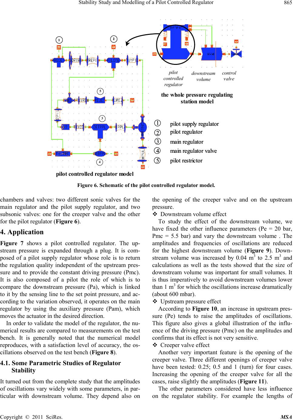
Stability Study and Modelling of a Pilot Controlled Regulator 868
sensing lines, the opening of the antipumping valve. This
feature has been confirmed by measurements and simu-
lations.
5. Conclusions
The final objective o f the study presented in this paper is
to improve the process control of the pressure regulator
that is to define the operating conditions that maintain a
constant set pressure at small enough oscillations within
tolerance field. For that purpose, numerical and experi-
mental approaches have been performed.
The comparison of calculations and measurements, has
confirmed the relevance of the modelling. From a quali-
tative and a quantitative point of view, the calculations
are in good agreement with experiments. Generally, the
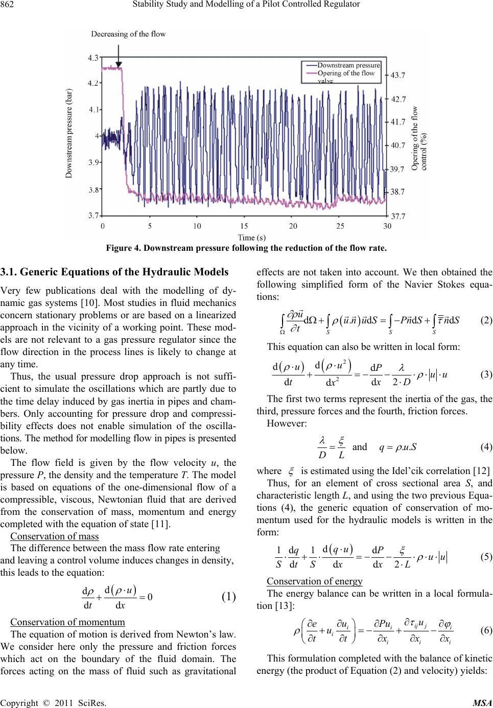
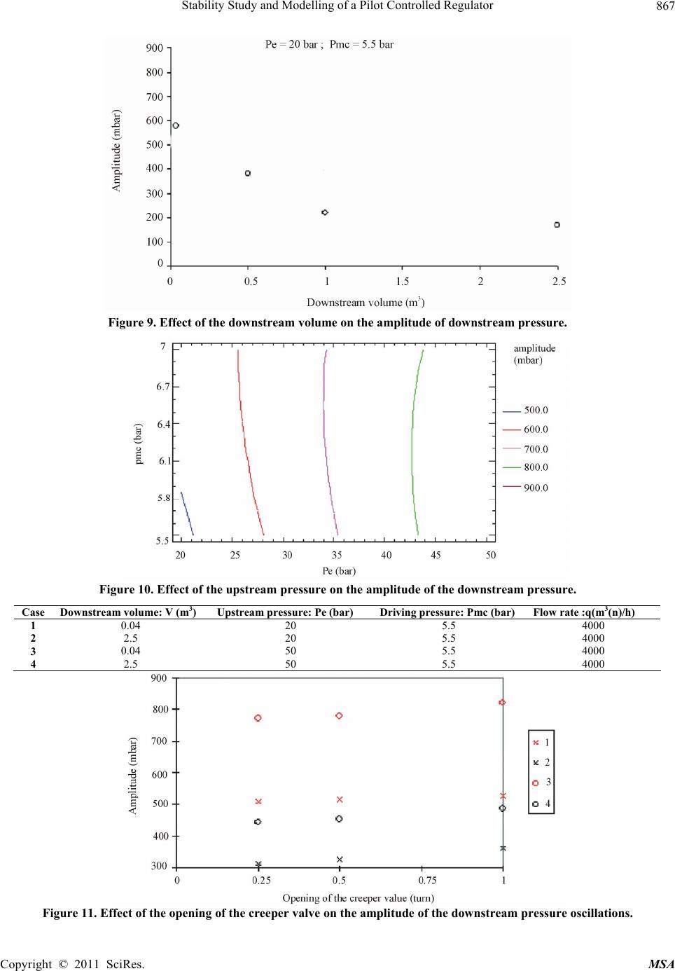
amplitude of oscillations increases dramatically for small
volumes (V = 0.04 m3) and higher upstream pressure. As
regards to the other parameters such as opening of
creeper valve and driving pressure, their influence on the
oscillation downstream pressure is not very sensitive.
Other adjustment parameters such as length of sensing
lines or opening of the antipumping valve, have only
marginal influences on the regulator stability.
6. Acknowledgments
The authors wish to express their indebtedness to Messrs.
MODE Laurent and DELENNE Bruno of the Research
and Development Division of Gaz De France for their
contributions toward the success of this work.
REFERENCES
[1] H. W. Earney, “Causes and Cures of Regulator Instatbil-
ity,” Fisher Controls International, Inc., Marshalltown,
1996.
[2] C. Carmichael, “Gas Regulators Work by Equalizing
Opposing Forces,” Pipe Line & Gas Industry, 1996, pp
29-33.
[3] B. Delenne, L. Mode and M. Blaudez, “Modelling and Si-
mulation of a Gas Pressure Regulator,” European Simula-
tion Symposium, Erlangen, Germany, 26-28 October 1999.
[4] B. Delenne and L. Mode, “Modelling and Simulation of
Pressure Oscillations in a Gas Pressure Regulator,” Pro-
ceedings of American Society of Mechanical Engineers,
Vol. 7, Orlando, 2000.
[5] Association Technique de l’Industrie et du Gaz en France,
Manuel pour le transport et la distribution du gaz, titre V
“Détente et Regulation du Gaz,” 1990.
[6] K. J. Adou, “Etude du Fonctionnement Dynamique des
Régulateurs-Detendeurs Industriels de Gaz,” Ph.D. Thesis,
Université Paris VI, Paris, 1989.
[7] F. Favret, M. Jemmali, J. P. Cornil, F. Deneuve and J. P.
Guiraud, “Stability of Distribution Network Governors
—R&D Forum Osaka Gas,” 1990.
[8] J. Goupy, “Plans D'expériences Pour Surface de Ré-
ponse,” Dunod, Paris, 2000.
[9] J. Goupy, “La Méthode des Plans d'expériences: Optimi-
sation du Choix des Essais et de L’interprétation des
Résultats,” Dunod, Paris, 1988.
[10] J. P. Schlienger and E. Bordenave, “Ecoulement Insta-
tionnaires de Gaz en Conduite,” 11 ème Congrès Interna-
tional du Gaz à Nantes, 1994.
[11] H. Schlichting, “Boundary Layer Theory,” McGraw Hill
Book Company, Auckland, 1979.
[12] Idel'cik, “Spravotchnik po Guidravlitcheskim Soprotiv-
leniam,” Memento des Pertes de charges, Gosenergoizdat,
Moscow, 1960.
[13] J. Taine and J. P. Petit, “Transfert de Chaleur; Thermique;
Ecoulement de Fluide,” Dunod, Paris, 1989.
[14] D. Y. Peng and D. B. Robinson, “A New Two-Constant
Equation of State,” Industrial & Engineering Chemistry
Fundamentals, Vol. 15, No. 1, 1976, pp. 59-64.
doi:10.1021/i160057a011
[15] H. W. Liepmann and A. Roshko, “Elements of Gas Dy-
namics,” John Wiley and Sons Inc., Hoboken, 1962.
[16] A. Jeandel, F. Favret, L. Lapenu and E. Lariviere,
“ALLAN. Simulat Ion, a General Tool for Model De-
scription and Simulation,” International Conference of
the International Building Performance Simulation Asso-
ciation, Adlaide, 16-18 August 1993.
[17] M. Nakhlé, “NEPTUNIX an Efficient tool for Large Size
Systems Simulations,” 2nd Internationnal Conference on
System Simulation, Lieges, Belgium, 3 December 1991.

Stability Study and Modelling of a Pilot Controlled Regulator869
NOMENCLATURE
Cf viscous damping (kg/s)
Cp specific heat at constant pressure (J/K/kg)
F
 
Friction force (N)
D pipe diameter (m)
e specific internal energy (J/kg)
g gravity acceleration (m/s2)
h specific internal enthalpy (J/kg)
K spring stiffness (N/m)
L pipe length (m)
M actuator mass (kg)
P pressure (Pa)
P0 absolute pressure (1,013 bar)
Pa downstream pressure (Pa)
Pe upstream pressure (Pa)
Pmc driving pressur e (Pa )
Pam auxiliary pressure (Pa)
R gas constant (J/kg/K)
s diaphragm area (m2)
S cross sectional area of pipe (m2)
T temperature (K)
V downstream volume (m3)
Z compressibility coefficient (-)
u fluid velocity (m/s)
x position along the pipe (m)
X actuator position (m)
 coefficient of thermal expansion (K-1)
 conductive heat flux (W/m2)
 pressure loss coefficient per length (-)
  dynamic viscosity (Pa.s)
 gas density (kg /m3)


  pressure loss coefficient (-) 

ij shear stress (second–1)
q mass flow rate ( kg/s or m3(n)/h :m3/h at normal conditions)
Note : normal conditions are taken in absolute pressure of 1,013 bar and temperature of 0˚C ( 273,15K)