 Open Journal of Mo dern Hydrology, 2011, 1, 1-9 doi:10.4236/ojmh.2011.11001 Published Online July 2011 (http://www.scirp.org/journal/ojmh) Copyright © 2011 SciRes. OJMH 1 ARMA Modelling of Benue River Flow Dynamics: Comparative Study of PAR Model Otache Y. Martins, M. A. Sadeeq, I. E. Ahaneku Department of Agricultural & Bioresources Engineering, Federal University of Technology, Minna, Nigeria E-mail: martynso_pm@yahoo.co.u k Received May 2, 2011; revised June 5, 2011; accepted July 6, 2011 Abstract The seemingly complex nature of river flow and the significant variability it exhibits in both time and space, have largely led to the development and application of the stochastic process concept for its modelling, fore- casting, and other ancillary purposes. Towards this end, in this study, attempt was made at stochastic model- ling of the daily streamflow process of the Benue River. In this regard, Autoregressive Moving Average (ARMA) models and its derivative, the Periodic Autoregressive (PAR) model were developed and used for forecasting. Comparative forecast performances of the different models indicate that despite the shortcom- ings associated with univariate time series, reliable forecasts can be obtained for lead times, 1 to 5 day-ahead. The forecast results also showed that the traditional ARMA model could not robustly simulate high flow re- gimes unlike the periodic AR (PAR). Thus, for proper understanding of the dynamics of the river flow and its management, especially, flood defense, in the light of this study, the traditional ARMA models may not be suitable since they do not allow for real-time appraisal. To account for seasonal variations, PAR models should be used in forecasting the streamflow processes of the Benue River. However, since almost all mechanisms involved in the river flow processes present some degree of nonlinearity thus, how appropriate the stochastic process might be for every flow series may be called to question. Keywords: Time Scale, Streamflow, Autoregressive Model, Fuzzy Cluster, Forecasting, Dynamics 1. Introduction Time series modelling for either data generation or fore- casting of hydrologic variables is an important step in planning and operational analysis of water resource sys- tems. But, providing good forecast functions for time dependent data has become a common problem. It is particularly acute in environmental and ecologic studies in which the ability to predict is closely allied to the suc- cessful allocation of the resources needed to control the environment. Operational hydrological forecasting and water resource management require efficient tools to provide accurate estimates of future river level condi- tions and meet real world demand. The use of stochastic time-series models for hydrologic forecasting has evolved greatly. Although many studies have given flow simulation considerable attention, it is important to rec- ognise that simulation is not an end in itself but rather a means to an end, the end being an optimal water resource design. Despite some notable applications and case stud- ies [1], relatively few studies have reported on the use of flow simulation or stochastic modelling in general in solving engineering problems [2]. More attention needs to be given to the uses of synthetic data, such as using the data with optimizing techniques to obtain optimal operating policies for storage or a set of storages. In the context of the above, stochastic linear models are fitted to hydrologic data for two main reasons: to enable forecasts of the data one or more time periods ahead to allow for the generation of sequences of syn- thetic data. In the same context, deterministic models are of importance in forecasting flows over very short time intervals such as hours or even days. But even in these situations if the parameters of a deterministic model have no physical interpretation and cannot be measured in the field, a deterministic model offers few advantages over a stochastic model [3]; since probability limits for fore- casts may readily be obtained, there may be advantages in using a stochastic model. Stochastic streamflow mod- els are often used in simulation studies to evaluate the likely future performance of water resources systems. Several stochastic models have been proposed for mod-  2 O. Y. MARTINS ET AL. elling hydrological time series and generating synthetic streamflows. These include Autoregressive Moving Av- erage (ARMA) models [4], disaggregation models [5], models based on the concept of pattern recognition [6]. Most of the time-series modelling procedures fall within the framework of multivariate autoregressive moving average (ARMA) models. Generally, Autoregressive (AR) and Autoregressive Integrated Moving Average (ARIMA) models have an important place in the stochastic modelling of hydrologic data. Such models are of value in handling what might be described as the short-run problem; that of modelling the seasonal variability in a stochastic flow series. In recent years, their importance to practical water resource prob- lems has been over-shadowed by more sophisticated types of models that are designed to preserve long-run dependencies, perhaps of the order of decades, in hydro- logic series. In most of these models, the Hurst h has been used to characterize the long-run dependencies. Although the long-run problem is important, the short- run problem, perhaps of the order of months to a few years, is important, too. Thus, as river flow dynamics at some time-space scales are not as irregular and complex as those at other time-space scales, the need and appro- priateness of the stochastic process concept for ‘every’ river flow, and hydrologic and geomorphic series calls for a second look at the totality of the whole assertion. In view of these conflicting paradigms, the question of whether a given river (or any hydrologic and geomorphic) series can be modelled appropriately by stochastic me- thods underscores the premise of this study. Considering all of this, the focus of the study is to model the daily flow sequence of the Benue River using Autoregressive Integrated Moving Average (ARIMA) and its two de- rivatives, the ARMA and the Periodic Autoregressive (PAR) models. Here, the feature of interest is to investi- gate the suitability of either model on the basis of some selected forecast performance criteria. 2. Materials and Methods 2.1. Hydrology of the Benue River The Benue River is the major tributary of the Niger River. It is approximately 1,400 km long and almost navigable during the rainy season (between July and Oc- tober). Hence, it is an important transportation route in the regions it flows through. Its headwaters rises in the Adamawa Plateau of the Northern Cameroon, flows into Nigeria south of the Mandara Mountains through the east-central part of Nigeria before entering the Niger River at Lokoja (Figure 1(a)). The wide flood plain is used for agriculture, with main crops being sugar cane (a) (b) Figure 1. (a) Map of Nigeria showing Benue River and its traverse; (b) General hydrologi c al y e a r flow regime. and rice. There is only one high-water season because of its southerly location; this normally occurs from May to October, while on the other hand, the low-water period is from December to June. Figure 1(b) explains the hydro- logical flow regime of the Benue River in line with the general climatic pattern. There are definite wet and dry seasons which give rise to changes in river flow and sa- linity regimes. The flood of the Benue River (upper, middle, and downstream) lasts from July to October, and sometimes up to early November. 2.2. Data Base Management In this study, historical time series for gauging stations at the base of the Benue River (i.e., Lower Benue River Basin) at Makurdi (7˚44′N, 8˚32′E) was used. A total of 26 years (1974-2000) water stage and discharge data were collected. A shorter time scale was considered for Copyright © 2011 SciRes. OJMH  O. Y. MARTINS ET AL. 3 the modelling and forecasting. To this end, daily average discharges were used only. 2.3. ARMA Modelling of the Daily Flows The procedure of fitting deseasonalised ARMA models to daily streamflow as used in this study involves two basic steps; i.e., deseasonalisation and ARMA model construction. To do this, the flow series was logarithmi- cally transformed and deseasonalised by subtracting the seasonal mean values and dividing by the seasonal stan- dard deviations of the logarithmic transformed series. To alleviate the stochastic fluctuations of both the daily and monthly means and standard deviations, they were smoothened by the first 8 Fourier harmonics respectively before being used for standardisation. To broaden the choices of the models in the modelling exercise, the pos- sibility of the traditional autoregressive integrated mov- ing average (ARIMA) model was examined. Unlike the deseasonalisation pre-processing method, the logarithmic transformed flow series was differenced before fitting the appropriate ARIMA model. The objective is to appraise the impact the pre-processing may have on the overall forecasting results for the respective models adopted. (a) (b) Figure 2. ACF of residuals from: (a) ARMA (20,1), and (b) ARIMA (8,2,3) models. Based on the Autocorrelation function (ACF) and Par- tial Autocorrelation function (PACF) structures of the flow series as well as the model selection criterion AIC, an ARMA (20,1), ARIMA (8,2,3) were fitted to the flow series. The parameters were estimated using the arima. mle function in S-Plus version 6 (Insightful Cooperation, 2001) software. In order to examine the goodness of fit of the ARMA (20,1), ARIMA (8,2,3) models respec- tively, the ACF of the residuals from the models were inspected. The ACF plots in Figure 2 show that there is no significant autocorrelation left in the residuals from both ARMA-type models. The adequacy of the models was further examined by using Ljung-Box test on the residual series. The Ljung-Box test results for ARMA (20,1), ARIMA (8,2,3), are shown in Figure 3. The p- values’ exceedance of 0.05 indicates the acceptance of the null hypothesis of model adequacy at the 5% signifi- cance level. 2.4. PAR Model Building A lot of contrasting difficulties are usually encountered in the development of different types of PAR models; for instance, model order, lose of generality, and the over- whelmingly burdensome and practically infeasible com- putation of compatibility between neighbouring days. Because of this, the method for fitting PAR model based on cluster analysis as espoused by Wang [7] and Otache [8] was adopted. The fuzzy clustering method was ap- plied to partition the days over an annual cycle in order to build the PAR model. The Fuzzy Clustering Method (FCM) approach partitions a set of n vectors , j j , into c fuzzy clusters; this implies that each data point belongs to a cluster to a degree specified by a membership grade ij between 0 and 1. Thus, a matrix U consisting of the elements ij can be defined based on the assumption that the summation of degrees of be- longing for a data point is equal to 1, i.e., 1i 1,, n uu 1 ij u c , j1, ,n . The objective of the FCM algorithm is to find c cluster centers such that the cost functions of dis- similarity (or distance measure) are minimized. The cost function is defined by 2 111 ,, ,cn m c ij ijij Uv vud (1) where, vi is the cluster center of the fuzzy group i; iji j dvx is the Euclidean distance between the ith cluster and the jth data point, and m ≥ 1 is a weighting exponent, taken as 2 here. The necessary conditions for Equation (1) to reach minimum are: 1 1 nm ij j j inm ij j ux vu (2) Copyright © 2011 SciRes. OJMH  O. Y. MARTINS ET AL. Copyright © 2011 SciRes. OJMH 4 (a) (b) Figure 3. Ljung-Box lack-of-fit tests for: (a) ARMA (20,1), and (b) ARIMA (8,2,3) models. Figure 4. Membership grades of the days over the year for the daily streamflow base d on fuzzy c lustering. and 1 21 1 m cij ij kkj d ud (3) In partitioning the days over the year with the cluster- ing approach, the raw average daily discharge data and the autocorrelation values at different lag times, say 1 - 10 days were used. The discharge data and the autocor- relation coefficients were organized as a matrix X of size where N is the number of years and 10 the autocorrelation values at 10 lags. To eliminate the influence of large differences among data values on the cluster result, the daily discharges were first logarithmi- cally transformed before carrying out the cluster analysis. Figure 4 shows the FCM clustering result. The entire daily discharge over the annual cycle was partitioned into three, basically conforming to the flow dynamics which is made up of low, medium, and high flows. The medium flow regime is a watershed or rather, the transi- tion between the low and high flows. Based on the parti- tioning results, one AR model was fitted to a partition. Before fitting the respective AR models, the daily streamflow series was deseasonalised. The orders of the AR models were determined according to AIC criterion [9], with the PACF acting as a basis for the model choices. The partitioning of the daily streamflow in terms of days over an annual cycle is shown in Table 1. Based on the minimum AIC, Table 2 shows the orders of the AR models for each partition while Table 3 indicate the concise definition of each partition in terms of the intrin- sic flow pattern. Collectively, the respective AR models constitute the PAR model. During the forecasting proc- ess, a specific AR model is applied depending on what season’s partition the date to be forecasted is in. 10 365N 2.5. Forecast Performance Measures Since forecast accuracy is best assessed by retrospective comparison of forecasts actually made or that which have been made, and the values observed during the forecast period, the following measures were used to evaluate model performances in the respective cases. Mean Absolute Error: 1 1n ii i AEQ Q n (4) Mean Absolute Percentage Error: 1 1ii n ii QQ MAPE nQ (5)  O. Y. MARTINS ET AL. 5 Root Mean Squared Error: 2 1 1 2 n ii i RMSEQ Q (6) Mean Squared Relative Error: 2 1 1n ii i i SREQ QQ n (7) Coefficient of Efficiency: 2 n 1ii iQQ 2 1 1n i i CE QQ (8) Coefficient of Determination: 2 1 22 11 n ii i nn ii ii QQQQ QQ QQ (9) Seasonally Adjusted Coefficient of Efficiency: 2 ii QQ 1 1 n i SACE 2 1 n im iQQ (10) Table 1. Partitioning of days based on FCM method. Partition 1 2 3 Day span 1-55, 268 - 365 56 - 105, 225 - 267 106 - 224 Table 2. Selected AR orders for the PAR model according to minimum AIC value. Partition 1 2 3 AIC 15 9 4 Table 3. Flow partitions and respective definition of flow pattern. Partition 1 2 3 Flow pattern Low flows Moderately high flows High flows where, Q and i are the n modelled and observed flows respectively; QQ and are the mean of the ob- served and modelled flows respectively and Q modmis (mod is the modulus, an operator used for calculating the remainder) is the season, ranging from 0 to S - 1; and S is the total number of season. The forecast exercise was done by using the models developed. In all the cases, the forecast horizon covers a two-year period; i.e., the last two years. It suffices to note that model building was on a rolling-forward basis. 3. Results and Discussion The forecast results were evaluated based on the stated measures of performance for each model under differing flow regimes as appropriate; namely, Wet (April-Octo- ber), and Dry (November-March).The evaluation results for 1 to 10-day ahead forecasts with the ARMA(20,1) are listed in Tables 4-6; ARIMA (8,2,3) in Tables 7-9, and PAR in Tables 10-12. Based on the performance statis- tics, the following observations can be made. In terms of the values of CE, it is obvious that both the ARMA (20,1), ARIMA (8,2,3), and PAR models indi- cate that satisfying forecasts can be achieved for lead times up to 10 days considering the whole year; that is, there is a possibility of making long-term forecasts of the streamflow process with the respective models. But con- cisely, this shows how much the CE statistic can fla- grantly exaggerate the forecast accuracy of the model; SACE statistic in contrast, indicates the contrary. Using a threshold of ≥ 0.9 [10], the SACE statistic shows that with the ARMA (20,1), satisfactory forecast can be ob- tained for up to a 10-day ahead lead time, and for ARIMA (8,2,3), it is 5 days; whereas with the PAR model, it is around 7 days. Realistically, baring model uncertainty resulting from problems of externalities (say, data quality problems, data size, non-stationarity and seasonality issues), based on the SACE statistic, reliable forecasts can plausibly be made up to a lead time of 7 days. It is important to note that there is obvious presence of significant seasonal variation in forecast accuracy. The forecast accuracy for dry season is relatively much higher than that of the wet season. Using the MAE statis- tic (threshold value, say, ≤ 150), with the ARMA (20,1), satisfactory forecasts on the average, can be made for up to 3 - 5 days, that is for both wet and dry season. On the same basis, the performance of the ARIMA (8,2,3) is abysmal for the wet season period; in the dry season pe- riod, reliable forecasts are possible for at most 4 days while with the PAR model, around 3 - 6 days for both wet and dry season periods. When assessing the per- formance of a streamflow forecasting model, it is not only important to evaluate the average prediction error but also the distribution of prediction errors as shown by the results here. It is important to know whether the model is predicting higher flows badly or the lower agnitude flows badly, which may help in further refin- m Copyright © 2011 SciRes. OJMH  O. Y. MARTINS ET AL. Copyright © 2011 SciRes. OJMH 6 Table 4. Forecast performance of ARMA (20,1) model for Whole year (Daily flows). Lead MAE MAPE RMSE MSRE CE SACE 2 r 1 66.01 0.019 136.72 0.001 0.999 0.914 0.999 2 90.85 0.025 193.32 0.002 0.998 0.913 0.998 3 115.25 0.030 247.59 0.002 0.996 0.911 0.998 4 140.22 0.036 303.02 0.003 0.995 0.910 0.997 5 160.77 0.041 347.91 0.003 0.993 0.908 0.996 6 186.62 0.047 402.48 0.004 0.991 0.906 0.995 7 206.37 0.051 443.88 0.005 0.989 0.905 0.994 8 232.23 0.058 497.25 0.006 0.987 0.903 0.993 9 252.53 0.063 539.58 0.007 0.984 0.900 0.992 10 271.06 0.068 577.97 0.008 0.982 0.898 0.991 Table 5. Forecast performance of ARMA (20,1) model for Wet season (Daily flows). Lead MAE MAPE RMSE MSRE CE 2 r 1 84.05 0.023 146.24 0.002 0.999 0.999 2 113.90 0.029 202.53 0.002 0.998 0.999 3 143.61 0.034 256.17 0.003 0.997 0.998 4 173.25 0.040 312.30 0.003 0.995 0.998 5 196.60 0.044 355.70 0.004 0.994 0.997 6 228.18 0.051 412.46 0.005 0.992 0.996 7 251.23 0.055 453.29 0.005 0.991 0.996 8 283.70 0.062 509.38 0.007 0.989 0.994 9 308.34 0.067 553.07 0.008 0.987 0.994 10 330.57 0.072 592.29 0.009 0.985 0.993 Table 6. Forecast performance of ARMA (20,1) model for Dry season (Daily flows). Lead MAE MAPE RMSE MSRE CE 2 r 1 40.43 0.013 121.97 0.001 0.997 0.998 2 58.19 0.018 179.46 0.001 0.995 0.998 3 75.05 0.024 234.91 0.001 0.991 0.997 4 98.40 0.030 289.35 0.002 0.987 0.996 5 109.99 0.035 336.55 0.002 0.982 0.996 6 127.73 0.041 387.91 0.003 0.976 0.994 7 142.81 0.046 430.21 0.004 0.971 0.993 8 159.29 0.051 479.54 0.004 0.964 0.991 9 173.44 0.056 519.87 0.005 0.958 0.990 10 186.72 0.061 557.05 0.006 0.951 0.989 Table 7. Forecast performance of ARIMA (8,2,3) model for Whole year (Daily flows). Lead MAE MAPE RMSE MSRE CE SACE 2 r 1 72.53 0.023 114.73 0.001 0.999 0.914 0.999 2 138.67 0.043 215.35 0.003 0.997 0.912 0.999 3 206.90 0.064 321.16 0.005 0.994 0.909 0.997 4 276.83 0.085 430.53 0.010 0.990 0.906 0.996 5 347.88 0.106 541.99 0.015 0.984 0.900 0.994 6 420.33 0.127 656.66 0.022 0.977 0.893 0.991 7 493.59 0.148 772.39 0.030 0.969 0.886 0.989 8 568.38 0.170 892.39 0.039 0.958 0.877 0.985 9 644.18 0.192 1014.21 0.051 0.946 0.865 0.982 10 721.30 0.213 1139.19 0.063 0.932 0.852 0.978 ing the model. While both the CE and r2 values in all the instances considered are high, indicating the quality and explanatory power of the ARMA (20,1), ARIMA (8,2,3), and PAR models in the respective cases, the high values of MAE, especially for the wet season (high flow period) portray a different picture to the contrary. The ARMA (20,1), ARIMA (8,2,3) and PAR failed to adequately capture the high flow dynamics of the streamflow, thus stressing the need for incorporating exogenous inputs in the streamflow forecasting exercise. Generally, the statistical performance criteria, RMSE, r2, and CE are global statistics and do not provide any robust information on the distribution of errors; precisely, CE, MSRE, RMSE, MAE, and r2 are all measures that incorporate both systematic and random errors. For in- stance, it is noted that a CE value of zero indicates that the observed mean is as good a predictor as the model, hile a negative value implies that the observed mean is w  O. Y. MARTINS ET AL. Copyright © 2011 SciRes. OJMH 7 Table 8. Forecast performance of ARIMA (8,2,3) model for Wet season (Daily flows). Lead MAE MAPE RMSE MSRE CE 2 r 1 100.51 0.022 142.56 0.001 0.999 0.999 2 192.42 0.040 269.32 0.002 0.996 0.999 3 287.95 0.059 401.93 0.005 0.993 0.998 4 386.62 0.079 539.36 0.008 0.987 0.997 5 487.30 0.101 679.58 0.014 0.980 0.996 6 590.87 0.122 824.49 0.021 0.971 0.994 7 695.62 0.144 970.80 0.029 0.960 0.992 8 804.48 0.167 1123.59 0.040 0.946 0.990 9 915.02 0.191 1278.75 0.053 0.930 0.987 10 1028.61 0.215 1438.56 0.067 0.912 0.984 Table 9. Forecast performance of ARIMA (8,2,3) model for Dry season (Daily flows). Lead MAE MAPE RMSE MSRE CE 2 r 1 32.87 0.025 54.89 0.001 0.999 0.999 2 62.50 0.048 96.46 0.003 0.998 0.998 3 92.03 0.071 142.73 0.006 0.996 0.997 4 121.24 0.093 189.12 0.011 0.994 0.996 5 150.29 0.114 235.68 0.017 0.991 0.994 6 178.62 0.135 280.91 0.023 0.987 0.992 7 207.29 0.155 326.22 0.031 0.983 0.989 8 233.78 0.174 368.53 0.039 0.978 0.986 9 260.34 0.193 411.05 0.048 0.973 0.982 10 285.77 0.211 451.72 0.057 0.968 0.979 Table 10. Forecast performance of PAR model for Whole year (Daily flows). Lead MAE MAPE RMSE MSRE CE SACE 2 r 1 67.69 0.019 142.05 0.001 0.998 0.914 0.999 2 96.09 0.026 203.73 0.002 0.997 0.912 0.998 3 122.97 0.032 263.42 0.002 0.996 0.911 0.998 4 150.62 0.038 324.05 0.003 0.994 0.910 0.997 5 176.60 0.043 382.51 0.003 0.992 0.907 0.996 6 202.85 0.049 438.79 0.004 0.990 0.906 0.995 7 226.87 0.054 492.02 0.005 0.987 0.903 0.993 8 252.07 0.061 543.92 0.006 0.984 0.900 0.992 9 275.05 0.067 593.04 0.008 0.981 0.898 0.990 10 297.34 0.072 640.10 0.009 0.978 0.893 0.989 Table 11. Forecast performance of PAR model for Wet season (Daily flows). Lead MAE MAPE RMSE MSRE CE 2 r 1 84.49 0.023 150.60 0.002 0.999 0.999 2 117.42 0.028 210.92 0.002 0.998 0.999 3 148.28 0.034 268.75 0.003 0.996 0.998 4 179.69 0.039 328.64 0.003 0.995 0.997 5 209.27 0.043 386.83 0.004 0.993 0.997 6 239.33 0.049 443.29 0.004 0.991 0.996 7 267.08 0.053 497.01 0.005 0.989 0.995 8 296.31 0.060 549.47 0.007 0.987 0.994 9 323.05 0.065 599.42 0.010 0.984 0.992 10 349.06 0.070 647.43 0.010 0.982 0.991 a better predictor than the model [11]. But for hydro- logical time series that often exhibit strong seasonality, the general concern is whether the model is better than seasonal mean values of the series rather than the overall observed mean. This phenomenon cannot adequately be addressed by CE as in Equation (8); similarly, it is noted that the value of CE calculated for a whole year is higher than the average of CE values calculated for separate seasons, which illogically implies that the model per- formance for the whole year is better than for most sepa- rate seasons [7]. These problems arise from the inade- quacy of the definition of CE in dealing with seasonal processes. Basically, CE’s definition is premised on the assumption that the process of interest is stationary [12]; but, hydrological time series usually exhibit strong sea- sonality. It is interesting to note that when strong season- ality exists, especially, when the mean value changes ith season, for most of the seasons (such as days or w 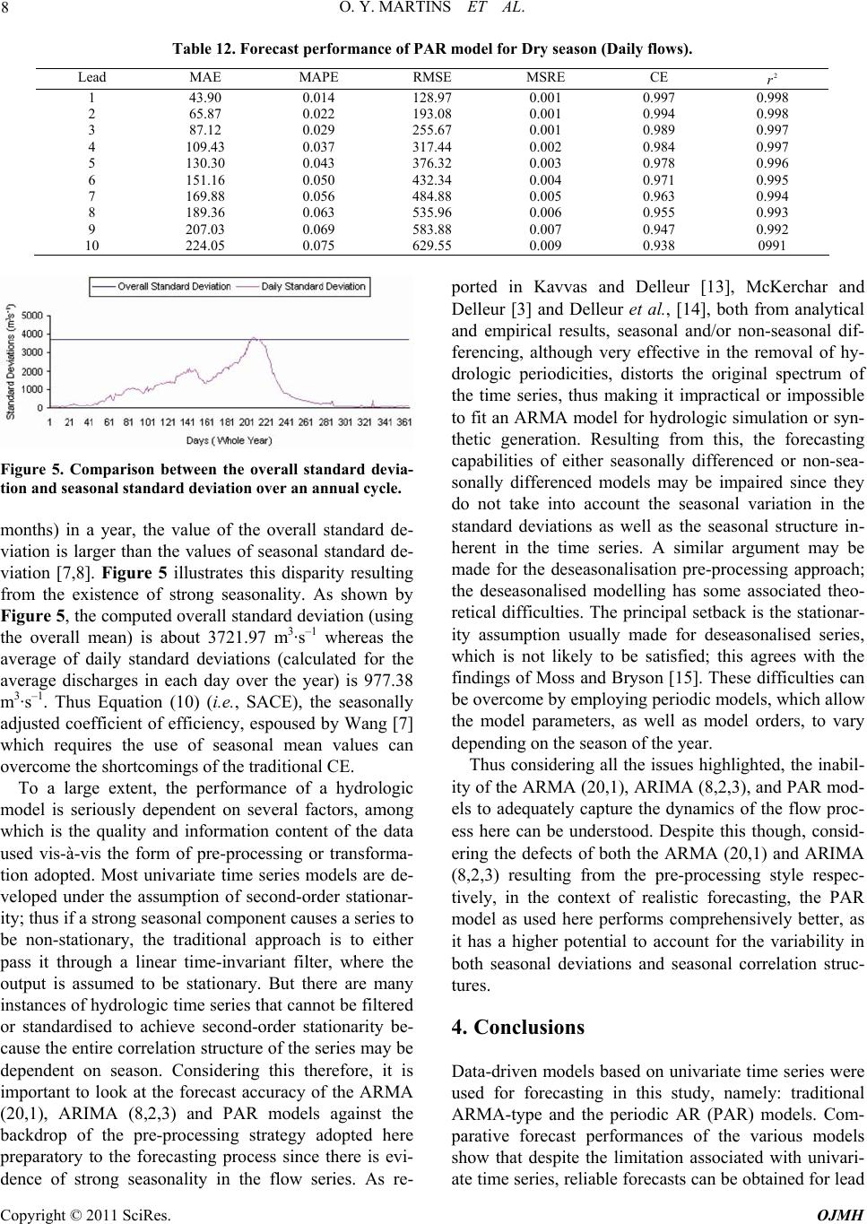 O. Y. MARTINS ET AL. Copyright © 2011 SciRes. OJMH 8 Table 12. Forecast performance of PAR model for Dry season (Daily flows). Lead MAE MAPE RMSE MSRE CE 2 r 1 43.90 0.014 128.97 0.001 0.997 0.998 2 65.87 0.022 193.08 0.001 0.994 0.998 3 87.12 0.029 255.67 0.001 0.989 0.997 4 109.43 0.037 317.44 0.002 0.984 0.997 5 130.30 0.043 376.32 0.003 0.978 0.996 6 151.16 0.050 432.34 0.004 0.971 0.995 7 169.88 0.056 484.88 0.005 0.963 0.994 8 189.36 0.063 535.96 0.006 0.955 0.993 9 207.03 0.069 583.88 0.007 0.947 0.992 10 224.05 0.075 629.55 0.009 0.938 0991 Figure 5. Comparison between the overall standard devia- tion and seasonal standard deviation over an annual cycle. months) in a year, the value of the overall standard de- viation is larger than the values of seasonal standard de- viation [7,8]. Figure 5 illustrates this disparity resulting from the existence of strong seasonality. As shown by Figure 5, the computed overall standard deviation (using the overall mean) is about 3721.97 m3·s–1 whereas the average of daily standard deviations (calculated for the average discharges in each day over the year) is 977.38 m3·s–1. Thus Equation (10) (i.e. , SACE), the seasonally adjusted coefficient of efficiency, espoused by Wang [7] which requires the use of seasonal mean values can overcome the shortcomings of the traditional CE. To a large extent, the performance of a hydrologic model is seriously dependent on several factors, among which is the quality and information content of the data used vis-à-vis the form of pre-processing or transforma- tion adopted. Most univariate time series models are de- veloped under the assumption of second-order stationar- ity; thus if a strong seasonal component causes a series to be non-stationary, the traditional approach is to either pass it through a linear time-invariant filter, where the output is assumed to be stationary. But there are many instances of hydrologic time series that cannot be filtered or standardised to achieve second-order stationarity be- cause the entire correlation structure of the series may be dependent on season. Considering this therefore, it is important to look at the forecast accuracy of the ARMA (20,1), ARIMA (8,2,3) and PAR models against the backdrop of the pre-processing strategy adopted here preparatory to the forecasting process since there is evi- dence of strong seasonality in the flow series. As re- ported in Kavvas and Delleur [13], McKerchar and Delleur [3] and Delleur et al., [14], both from analytical and empirical results, seasonal and/or non-seasonal dif- ferencing, although very effective in the removal of hy- drologic periodicities, distorts the original spectrum of the time series, thus making it impractical or impossible to fit an ARMA model for hydrologic simulation or syn- thetic generation. Resulting from this, the forecasting capabilities of either seasonally differenced or non-sea- sonally differenced models may be impaired since they do not take into account the seasonal variation in the standard deviations as well as the seasonal structure in- herent in the time series. A similar argument may be made for the deseasonalisation pre-processing approach; the deseasonalised modelling has some associated theo- retical difficulties. The principal setback is the stationar- ity assumption usually made for deseasonalised series, which is not likely to be satisfied; this agrees with the findings of Moss and Bryson [15]. These difficulties can be overcome by employing periodic models, which allow the model parameters, as well as model orders, to vary depending on the season of the year. Thus considering all the issues highlighted, the inabil- ity of the ARMA (20,1), ARIMA (8,2,3), and PAR mod- els to adequately capture the dynamics of the flow proc- ess here can be understood. Despite this though, consid- ering the defects of both the ARMA (20,1) and ARIMA (8,2,3) resulting from the pre-processing style respec- tively, in the context of realistic forecasting, the PAR model as used here performs comprehensively better, as it has a higher potential to account for the variability in both seasonal deviations and seasonal correlation struc- tures. 4. Conclusions Data-driven models based on univariate time series were used for forecasting in this study, namely: traditional ARMA-type and the periodic AR (PAR) models. Com- parative forecast performances of the various models show that despite the limitation associated with univari- ate time series, reliable forecasts can be obtained for lead  O. Y. MARTINS ET AL. 9 times, one to 5-day-ahead on the average for all the models used. The forecast results also brought to the fore the inadequacy of the traditional ARMA model. It was unable to robustly simulate high flow regimes unlike the periodic AR (PAR). Because of this, it is imperative that in order to account for seasonal variations, PAR models should be used in forecasting the daily streamflow proc- ess of the Benue River. However, the stochastic model- ling does show that the ARMA type models could be used as preliminary models for the basis of understand- ing the dynamics of the streamflow process. In the light of the results obtained in this study, suffice it to note that one limitation of this study is smallness of the data size used for modelling the streamflow process. Thus, to enhance the performance of the models and es- tablish the generality of the conclusions drawn, it is strongly recommended that larger data size be used, and too, explanatory exogenous variables (e.g. precipitation) be included during the modelling exercise, i.e., multi- variate modelling. To this end, in order to improve the accuracy of long-range forecasts, investigation of the linkage between streamflow processes and ancillary hy- droclimatic factors would be inevitable. In addition, since predictability is an important aspect of the dynam- ics of hydrological processes, though not considered in this study, a definition of the predictability of the stream- flow processes is a necessity; at least to put forward a predictable horizon for the entire respective flow dy- namics. 5. References [1] M. B Fiering and B. J. Jackson, “Synthetic Streamflows,” Water Resources Mongraph, Amer Geophysical Union, Washington, D.C, Vol. 1, 1971, p. 98. [2] T. O’Donnell, M. J. Hall and P. E. O’Connell, “Some Applications of Stochastic Hydrologic Models,” Pro- ceedings of the International Symposium on Mathemati- cal Modelling Techniques in Water Resource Systems, Environ, Ottawa, May 1972. [3] A. I. McKerchar and J. W. Delleur, “Application of Sea- sonal Parametric Linear Stochastic Models to Monthly Flow Data,” Water Resources Research, Vol. 10, No. 2, 1974, pp. 246-254. doi:10.1029/WR010i002p00246 [4] G. E. P. Box and G. M. Jenkins, “Time Series Analysis Forecasting and Control,” Holden-Day Press, San Fran- cisco, 1976. [5] R. D. Valencia and J. C. Schaake, “Disaggregation Proc- esses in Stochastic Hydrology,” Water Resources Re- search, Vol. 9, No. 3, 1973, pp. 580-585. doi:10.1029/WR009i003p00580 [6] U. S. Panu and T. E. Unny, “Extension and Application of Feature Prediction Model for Synthesis of Hydrologic Records,” Water Resources Research, Vol. 16, No. 1, 1980, pp. 77-79. doi:10.1029/WR016i001p00077 [7] W, Wang, “Stochasticity, Nonlinearity and Forecasting of Streamflow Processes,” Deft University Press, Amster- dam, 2006, pp. 1-17, ISBN 1-58603-621-1. [8] M. Y. Otache, “Contemporary Analysis of Benue River flow Dynamics and Modelling,” Unpublished Ph. D Dis- sertation, Hohai University, Nanjing, 2008. [9] H. A. Akaike, “New Look at Statistical Model Identifica- tion,” IEEE Transactions on Automatic Control, Vol. 19, No. 6, 1974, pp. 716-722. doi:10.1109/TAC.1974.1100705 [10] A. Y. Shamseldin, K. M. O’Connor and G. C. Liang, “Methods for Computing the Output of Different Rain- fall-Runoff Models,” Journal of Hydrology, Vol. 179, 1997, pp. 203-229. doi:10.1016/S0022-1694(96)03259-3 [11] B. P. Wilcox, W. J. Rawls, D. L. Brakensiek and J. R. Wight, “Predicting Runoff from Rangeland Catchments: A Comparison of Two Models,” Water Resources Re- search, Vol. 26, No. 10, 1990, pp. 2401-2410. doi:10.1029/WR026i010p02401 [12] R. J. Bhansali, “Autoregressive Estimation of the Predic- tion Mean Squared Error and an R2 Measure: An Appli- cation,” In: D. Brillinger, et al., Eds., New Directions in Time Series, Part I, Springer-Verlag, New York, 1992, pp. 9-24, [13] M. L. Kavvas and J. W. Delleur, “Removal of Peri- odicities by Differencing and Monthly Mean Subtrac- tion,” Journal of Hydrology, Vol. 26, 1975, pp. 335-353. doi:10.1016/0022-1694(75)90013-X [14] J. W. Delleur, P. C. Tao and M. L. Kavvas, “An Evalua- tion of the Practicality and Complexity of Some Rainfall and Runoff Time Series Models,” Water Resources Re- search, Vol. 12, No. 5, 1976, pp. 953-970. doi:10.1029/WR012i005p00953 [15] M. E. Moss and M. C. Bryson, “Autocorrelation Structure of Monthly Streamflows,” Water Resources Research, Vol. 10, No. 4, 1974, pp. 737-744. doi:10.1029/WR010i004p00737 Copyright © 2011 SciRes. OJMH
|