Energy and Power En gi neering, 2011, 3, 366-375
doi:10.4236/epe.2011.33047 Published Online July 2011 (http://www.SciRP.org/journal/epe)
Spatial Reactor Dynamics and Thermo Hydraulic Behavior
Simulation of a Large AGR Nuclear Power Reactor in
Response to a Reactivity Step Change Disturbance
Mohammad Reza Ansari, Reza Marzooghi
Mechanical Engineering Department, Faculty of Engineering, Tarbiat Modares University, Tehran, Iran
Received January 22, 2011; revised March 13, 2011; accepted Marc h 25, 2011
Abstract
In this article, two-dimensional partial differential equations with time representation of nuclear power reac-
tor kinetics are considered for spatial reactor dynamics and thermo hydraulic behavior analysis of a large
thermal advanced gas cooled reactor (AGR) type used for nuclear power generation. The equations include
the neutron flux equation and delayed neutron precursor concentration, together with taking into account the
equations to represent the thermo hydraulic behavior of the fuel, coolant and moderator temperatures. These
equations are solved numerically using the finite difference method. For time propagation, an implicit
method is applied. The desired initial condition for the reactor to stay at stable critical condition is estab-
lished by finding the correct value of reactivity. The reactivity disturbance effect in the reactor is studied for
different cases and presented for high reactivity values. The model was developed for the analysis of a large
AGR with 2000 MWe for future power generation. The results show that the model not only behaves stably
but also predicts the results physically for all the various parameters.
Keywords: Nuclear Reactor, AGR; Reactivity, Neutron Flux, Thermo Hydraulics
1. Introduction
Nuclear power stations play an important role in electric-
ity generation in industrial countries. Nuclear energy is a
clean and cheap energy source after renewable energy
sources, such as solar and hydraulic energy. Thus, for
industrial development, progress in nuclear power reac-
tors is essential. Advanced gas cooled reactors (AGR)
and the next generation high temperature gas cooled re-
actors (HTGR) are safe with respect to their moderator
and cooling materials and can generate a high amount of
energy; these types of nuclear reactors are desired for
high capacity nuclear power plants.
Nuclear reactor simulations are conducted for analysis
of reactor behavior. There are some computer codes that
have been developed by universities or research estab-
lishments in order to predict flow regimes, hydro dy-
namical instability, reactor kinetics, etc. These computer
codes (analyzers) include MINCS, PHOENICS, TRAC,
RELAP5, and others, and they not only predict the opti-
mized criteria for the thermo hydraulic condition for nu-
clear reactors but also fill in the gaps between the scarce
experimental results that have been found by different
research sources and obtained under substantially differ-
ent conditions. These codes have some capabilities and
limitations that have been discussed by Wulff [1] and
Physical Benchmarking Exercise [2]. RELAP5 has been
used massively for nuclear reactor modeling. Compari-
son of results obtained by RELAP5 modeling and ex-
perimental data collected by Groudev [3] for pressurized
water reactors (PWR) of VVER440/V230 type showed
that the analysis using this computer code is valid. Be-
cause such codes are not easily accessible, especially for
developing countries, modeling of the nuclear reactors
with more accurate mathematics and higher physics is
required to predict more precise simulation results.
Arab-Alibeik et al. [4,5] modeled a PWR reactor.
Their model is one-dimensional and includes five differ-
ential equations. They include the neutron flux equation
without a diffusion term, the six group delayed neutron
equation, energy conservation equations for fuel tem-
perature and an energy conservation equation for the
cooling flow. They also used fuel and moderator feed-
back coefficients in the model.

M. R. ANSARI ET AL.367
Marseguerra et al. [6] used the point kinetics neutron
flux equation with thermal equilibrium equations for the
reactor core. In their model, the neutron diffusion term
was omitted from the neutron flux equation. They con-
sidered six groups for the delayed neutron equations.
Weyfeng et al. [7] presented a three-dimensional model
that based on a 200 MW mina tour reactor with a thermal
pool reactor. Their model included the neutron flux
equation, one group equation including a neutron diffu-
sion term, delayed neutrons, the cooling flow thermal
equilibrium equation and one state equation for the effect
of control rod replacement on the neutron flux. Sadek et al.
[8] used a one-dimensional second order parabolic equa-
tion to model the nuclear reactor, including neutron flux
but without delayed neutrons and thermo hydraulic
terms.
In this article, the two-dimensional neutron flux equa-
tion is considered for the neutron spatial distribution to-
gether with equations to represent the dynamic behavior
of the fuel, coolant and moderator temperatures. In this
model, which has been applied to an AGR type reactor,
the cooling temperature is different than the moderator
temperature and is included in the equations definition.
This model has one more differential equation with re-
spect to the PWR model that was presented by other re-
searchers. The present model will consider symmetric
and anti-symmetric reactivity inlet disturbances and their
effect on nuclear reactor behaviors.
2. Modeling
2.1. Governing Equations
Nuclear reactor kinetic equations are declared by neu-
tronic and thermo hydraulic equations to describe the
dynamic behavior of the reactor core. Nuclear reactor
neutronic equations include prompt and delayed neutrons.
The neutron flux differential equation is as follows (Sta-
cey [9] and Glasstone, et al. [10]):

2
1
a
kC
t





 
 (1)
The one group delayed neutron precursor concentra-
tion equations are
d
da
Ck
tC




 (2)
In the one group delayed neutrons equations, the six
groups of delayed neutrons are averaged, and only one
variable is used instead of six variables. The average one
group delayed neutron and one-energy group equation is
written as
6
1
6
1
1
ii
i
ii
i
CC









(3)
To solve the above equations, the variables are nor-
malized as
0
0
P
C
DC




(4)
The normalized equations of the neutron flux and de-
layed neutron become as follows:

22
d
d
P
M
PP
tD
 
 (5)

d
d
DPD
t
 

(6)
P is the normalized power, and the time constant of
normal power and migration area are obtained as
2
1
a
a
k
Mk




 

(7)
Reactor reactivity will be affected by the fuel and
moderator temperature feedback coefficients. The reac-
tivity feedback formula is as follows:



00fffmmm
TT TT    

0
(8)
Fuel, cooling and moderator temperatures can be
found from the following differential equations:


 

11 1
21 2
32 2
d
d
d2
d
d
d
ffc
cfc mcpc
mmc
TECNPHT T
t
T
1
H
TT HTTMcTT
t
TECNPHT T
t



 





 



(9)
The above equations can be derived by considering the
thermal equilibrium between the fuel, cooling and mod-
erator temperatures. The fuel and moderator tempera-
tures are varied by the power that is released from the
nuclear energy generated from neutron production. The
fuel rods and moderator portion from the generated
power E1 and E2, respectively, as follows:
12
1EE

 (10)
The cooling temperature is assumed to be the average

M. R. ANSARI ET AL. 368
of the inlet and the outlet temperature of the reactor
21
2
c
TT
T  (11)
The mass flow rate is determined in such a way that
the cooling temperature is constant, which can be ob-
tained by assuming that the time variation of the cooling
temperature is equal to zero. The following equation can
be obtained for the cooling flow rate:



12
1
2
f
cm
pc
c
H
TT HTT
McTT
 

 (12)
2.2. Initial and Boundary Conditions
To solve equations, the initial condition for different
variables must be determined over the whole reactor
cross-section area. The power distribution in the reactor
at the initial condition is assumed to be a sinusoidal form,
as shown on Figure 1. The reactivity distribution is
found using the following equation:


11
,, ,,
nn nt
ijijij ij
PP 

 
0
(13)
 is a constant and is called the convergence coeffi-
cient. Its value can be found by trial and error. When the
right values of reactivity are found, it should be checked
in the model that the power stays at the initial condition
without changing when the computer program is run for
a long period of time. See Figure 2 for the normalized
power distribution after a long period of time (steady-
state condition). The other variable distributions were
found with respect to the power at the steady-state condi-
tion and are presented in Figures 3 to 7. The variables
values are high at the reactor center but decline to their
minimum values near the reactor boundaries.
0 2 4 6 8 10
0
2
4
6
8
10
0
0. 2
0. 4
0. 6
0. 8
1
x (m )
Initial Distribution of Normalized Power
y (m )
0. 55
0. 6
0. 65
0. 7
0. 75
0. 8
0. 85
0. 9
0. 95
Figure 1. Initial distribution of normalized power at the
reactor core cross -s ection.
0 2 4 6 8 10
0
2
4
6
8
10
0
0.2
0.4
0.6
0.8
1
x (m )
Steady St at e Nor ma l i zed Power Dist r ibut i on
y (m )
P
0.55
0.6
0.65
0.7
0.75
0.8
0.85
0.9
0.95
Figure 2. Normalized power distribution at the reactor
cross-section after using the right values of reactivity.
0246810
0
2
4
6
8
10
0
0.2
0.4
0.6
0.8
1
x ( m )
Steady Stat e Delayed Neutron G enerat i on Dist ribut i on
y ( m )
D
0.55
0.6
0.65
0.7
0.75
0.8
0.85
0.9
0.95
Figure 3. Initial values of delayed neutron distribution
across the reactor core.
0246810
0
2
4
6
8
10
420
440
460
480
500
x ( m )
Steady St at e Fuel Tem per at ur e Dis t r i but i on
y(m)
T
f
(

C)
440
450
460
470
480
490
Figure 4. Initial values of fuel temperature distribution
across the reactor core.
3. Solution Technique
To solve the governing equations numerically, the im-

M. R. ANSARI ET AL.369
0246810
0
2
4
6
8
10
380
385
390
395
400
x ( m )
Steady Stat e Coolant Temper at ure Dist r i but i on
y ( m )
T
c
(C)
382
384
386
388
390
392
394
396
Figure 5. Initial values of coolant temperature distribution
across reactor core.
0246810
0
2
4
6
8
10
385
390
395
400
405
410
x (m)
Steady St at e M odera tor Tem per at ure Dist r i but i on
y (m )
T
m
(

C)
388
390
392
394
396
398
400
402
404
406
Figure 6. Initial values of moderator temperature distribu-
tion across reactor core.
0246810
0
2
4
6
8
10
12
14
16
18
20
22
x (m )
Steady State Coolant M ass Fl ow Rate Dist r i buti on
y (m )
M (Kg/s)
14
15
16
17
18
19
20
21
Figure 7. Initial values of coolant flow rate distribution
across the reactor core.
plicit method was applied for differentiation because it
has higher numerical stability. The total differentiated
equations were solved using the Three Diagonal Matrix
Algorithm (TDMA) by considering the Alternative Di-
rection Implicit (ADI) method. Two set of equations,
including neutronic and thermo hydraulic equations,
were considered. The neutronic equations include the
normal power equation, delayed neutrons and tempera-
ture feedback on reactivity. The thermo hydraulic equa-
tions include the fuel, cooling and moderator tempera-
tures and the cooling flow rate. The two sets of equations
are affected mutually by the reactivity feedback equation,
and all of the equations must be solved together simulta-
neously. A square cross-section nuclear reactor is as-
sumed with 10 by 10-meter dimensions. The number of
meshes in the x and y directions are 21. Mesh independ-
ency was also considered with a different number of
meshes and increased up to 101 meshes in each direction.
The results generated from different runs of the computer
program showed that the differences are negligible. Thus,
the results obtained in the rest of the article depend on 21
meshes in each direction.
The second order partial derivatives of the neutron
flux equations were converted into differentiated form.
Each step of time was conducted in two half steps. In the
first half step of the time, the neutron flux equation was
solved implicitly in the x direction but explicitly in the y
direction. In the second half of the time step, the same
neutron flux equation was solved implicitly in the y di-
rection and explicitly in the x direction. Because of the
long mathematical manipulation and shortage of space,
only the final form of the obtained differentiated equa-
tions is presented below.
The neutron flux equation in the first half of the step
of time is

22
12 12
1,, ,
22
22 2
12
1,, 1,
22 2
2
,1
2
22
2
22
2
2
nn
i jijij
nn n
i jijij
nn
ij i
MM t
PP
tt xx
MM M
PP P
t xy y
MPD
t
y

 











 






 




n

(14)
The neutron flux equation in the second half of the
step of time is

22
11
,1, ,
22
22 2
112 12
,1 1,,
22 2
2
12
1,
2
22
2
22
2
2
nn
ijij ij
nn n
iji jij
nn
ij i
MM t
PP
tt
yy
MM M
PP P
t yx x
MPD
t
n
x

 





 












 





 

The normalized delayed neutron precursor concentra-
(15)

M. R. ANSARI ET AL. 370
tion equations are
11
,,
1
11
nn
ij ijij
t
DP
t






,
n
D
t
(16)
The equations representing fuel, coolant and modera-
tor temperatures are, respectively,
11 1 11
1,1, 1,,
111n 2
1,1 2,,2,
2
,,1
111 33
2,2 ,2,,
2
2
nnn n
fij cijijfij
nnn
f
ijij pcijmij
nn
ci ji jp
nnnn
cijmijij mij
HT HT ECNPT
tt
HTHHMc THT
t
TMcT
t
HTHTECNPT
tt



 








 






 

















(17)
The required coolant flow varies as







11nn 11
1,,2 ,,
1
,1
,1
2
nn
f
i jci jmi jci j
n
ij n
pcij
T
McT T





 (18)
Equations (13) to (17) were solved for each step of
tim
. Results
.1. Whole Reactor Cross-Section Disturbed by
nce the correct values of the different variables were
HT THT


e.
4
4Reactivity
O
established, the reactivity value was increased by 0.01
mN (mN is the reactivity unit used in the British nuclear
industry) over the entire reactor area after 0.1 seconds.
Figure 8 shows the transient response of the reactor with
respect to the reactivity change. The reactor power at the
middle point increased to about 25 times of the initial
state in just 0.7 seconds, then declined to 1.93 times the
initial value after 1.7 seconds and then increased slightly.
This behavior is the transient response of the reactor with
respect to the disturbances. The stable behavior of the
reactor starts after about 4 seconds. Figure 8 is plotted
for 5 seconds to demonstrate the reactor behavior at an
early time at the center of the reactor, and Figure 9 is the
continuation of the Figure 8 behavior at a longer time. It
also shows that the power increased gradually with time
and reached 8.2 times from 4.6 times the initial values in
45 seconds. The sudden increase of the reactor power in
Figure 8 was caused by prompt neutrons that were gen-
erated quickly by the reactivity disturbance response.
The second increase in power was because of the delayed
neutron generation. Figure 10 shows same behavior at
00.5 11.5 22.5 33.5 44.5 5
0
5
10
15
20
25
30
time (s)
P
Transi ent Response t o Reactivi ty St ep Dis tur bance
Figure 8. Nuclear reactor power response to uniform reac-
tivity disturbance at early time.
510 15 20 2530 35 4045 50
4.5
5
5.5
6
6.5
7
7.5
8
8.5
time (s)
P
Per m anent Respons e t o React iv i t y St ep Di s t ur bance
Figure 9. Nuclear reactor power response to uniform reac-
tivity disturbance at long period of time.
0 1 23 45 6 78 910
0
2
4
6
8
10
12
14
16
x ( m )
P
Response to React ivit y Step Di st ur ba nce
t = 0s
t = 0.5s
t = 5.0s
t = 50s
Figure 10. Power response to a uniform reactivity step change.

M. R. ANSARI ET AL.371
0246810
0
2
4
6
8
10
0
2
4
6
8
10
x ( m )
Response to Reacti vi t y Step Di st urbanse
y ( m )
P
1
2
3
4
5
6
7
8
Figure 11. Spatial power distribution to step change in re-
activity after 50 seconds.
00.5 11.5 22.5 33.5 44.5 5
2
4
6
8
10
12
14 x 10
-3
time (s)

Transient Response to Reactivity Step Disturbance
Figure 12. Transient response of reactivity after uniform
disturbance of reactivity in early period.
510 15 20 25 30 35 40 4550
2.5
3
3.5
4
4.5
5
5.5 x 10
-3
time (s)

Pe rm anent Response to Re activity Step Disturba nce
Figure 13. Transient response of reactivity after uniform
Figure 11
disturbance of reactivity in long period of time.
the center cross-section of the reactor core.
presents the reactor power after 50 seconds. It is inter-
esting that, because of the sharp power profile in the ini-
tial conditions, the early time power profile is sharp
(Figure 10 at a time of 0.5 sec), but, because of the high
difference of neutron flux between the center and the
boundaries, the power profile becomes almost uniform
over the whole reactor cross-section (Figures 10 and 11
at 50 seconds). Figure 12 for an early time and Figure
13 for a longer period of time show the reactivity tran-
sient behavior after it was increased intentionally. The
reactor power decreases and tends to stabilize the system
because of the negative reactivity feedback coefficient
effect. Figure 14 demonstrates the transient response of
the fuel, coolant and moderator temperatures on the reac-
tivity disturbance at an early time. The fuel temperature
increment is greater than the other temperatures, and
00.5 11.5 22.5 33.5 44.5 5
350
400
450
500
550
600
650
700
time (s)
T (C)
Transient Response to Reactivity Step Disturbance
T
f
T
c
T
m
Figure 14. Transient behavior of fuel, coolant and modera-
tor to reactivity step disturbance at early time.
510 15 20 2530 35 40 4550
300
400
500
600
700
800
900
1000
1100
1200
time (s)
T (

C)
P ermane n t Respo n se to Reactiv ity S tep Disturb ance
T
f
T
c
T
m
Figure 15. Transient behavior of fuel, coolant and modera-
tor to reactivity step disturbance at long period of time.

M. R. ANSARI ET AL. 372
ust
.2. One Node at Center of Reactor tivity
uring the previous section of the present paper, the
from 430˚C in equilibrium it increased to 685˚C in j
2.5 seconds. The temperature behavior is also presented
for longer periods of time in Figure 15. Because of the
higher power production, the fuel temperature increased
more with respect to moderator temperature. Because of
the greater time constant of the moderator, the moderator
temperature increase was lower than the fuel temperature.
The cooling temperature is a function of the fuel tem-
perature increment, but the cooling temperature incre-
ment was low because the cooling flow rate also in-
creased. The cooling temperature reached 507˚C from
380˚C for the initial value in 50 seconds. The fuel tem-
perature distribution in the reactor cross-section is pre-
sented in Figure 16 for different times, and the cooling
mass flow rate response to the uniform reactivity distur-
bance is presented in Figure 17.
4Cross-Section Disturbed by Reac
D
whole cross-section of the reactor core was disturbed by
the reactivity. In this section, only one node was dis-
turbed at the center of the core by a reactivity value of
0.1 mN (which is added to the initial value of the reactiv-
ity). The reactivity disturbance starts after 0.1 seconds.
The reactor transient response for power is presented in
Figure 18. Because of the high value of reactivity, the
reactor power increased sharply, but after about 0.78
seconds its value decreased to 0.16 times the initial value.
The oscillating behavior of the reactor decreased to a
stable value after around 15 seconds. The long-term be-
havior of the reactor power is presented in Figure 19.
The reactor power oscillation in Figure 18 was caused
by the fast generation of the prompt neutrons generated
0 123 4 5 6 7 8 910
400
500
600
700
800
900
1000
1100
1200
1300
1400
x (m )
T
f
(

C)
Response to React ivity St ep Di stur bance
t = 0s
t = 0.5s
t = 5.0s
t = 50s
Figure 16. Fuel temperature distribution across the reactor
core due to reactivity step change at different times.
05 1015 202530 35 40 45 50
10
15
20
25
30
35
40
45
50
55
60 Transie nt Response to Re a ctivity Step Disturbance
time (s)
M (Kg/s)
Figure 17. Coolant flow rate response due to reactivity step
change.
05 10 15
10
-1
10
0
10
1
10
2
10
3
10
4
time (s)
P
Transi ent Response to Reacti vi t y Step Distur bance
Figure 18. Power response to a point disturbance in reac-
tivity for 15 seconds.
15 20 25 3035 40 45 50
40
42
44
46
48
50
52
54
time (s)
P
Permanent Response to Reactivi t y St ep Dist urbance
Figure 19. Power response to a point disturbance in reac-
tivity up to 50 seconds.

M. R. ANSARI ET AL.373
reactivity disturbance. However, by the high amount of
the high value power production was damped and de-
creased by delayed neutron production. The reactor
power behavior was not only affected by the prompt and
delayed neutron productions and leakage but also con-
trolled by positive and negative reactivity feedback coef-
ficients due to the fuel and moderator temperatures. It
should be mentioned that the large value of the reactivity
introduced into reactor system is dangerous to the reactor
because it will generate very high power and fuel, mod-
erator and cooling temperature increases, as shown in
Figure 19. Such a high value temperatures will melt
down the reactor and possibly create a reactor explosion.
Our model cannot predict the melt down or reactor ex-
plosion (the equations do not contain the complicated
condition of the melt down or reactor explosion correla-
tions). However, it is intended to demonstrate and show
the responses of different parameters for a high value of
reactivity when put into operation intentionally. Then, the
reactor responses can be analyzed, and the model capa-
bilities and limitations can be considered. The reactor
responses were not only characterized physically (qualita-
tively) but also checked mathematically without any fail-
ure of the model developed (i.e., it remained stable nu-
merically). The results showed that, even for a high reac-
tivity, the model stayed stable numerically without facing
hard failure of the solution. Figure 20 presents the tran-
sient reactor behavior due to the reactivity step distur-
bance at different time levels, and Figure 21 shows the
power at the reactor cross-section at a time of 1.0 second.
The reactivity behavior for a period of 15 seconds is
shown in Figure 22, and that for longer period of time is
presented in Figure 23. Fuel, coolant and moderator tem-
perature behavior are presented in Figure 24 for an early
012345678910
10
-1
10
0
10
1
10
2
x ( m )
P
Response t o Tr ansient Respons e
t = 0s
t = 0.4s
t = 0.5s
t = 1.0s
t = 5.0s
x ( m )
y ( m)
P , t = 1 . 0s
10
Figure 20. Power distribution across the reactor at differen
times due to symmetric point reactivity disturbance. t
0 1 23 45 6 78 910
0
1
2
3
4
5
6
7
8
9
0. 2
0. 3
0. 4
0. 5
0. 6
0. 7
0. 8
Figure 21. Power distribution across the reactor at 1 secon
due to symmetric point reactivity disturbanc e . d
05 10 15
-0.08
-0.06
-0.04
-0.02
0
0.02
0.04
0.06
0.08
0.1
0.12
time (s)

Transient Response to Reactivity Step Disturbance
Figure 22. Transient response of reactivity due to symmet
ric point reactivity disturbance at early time. -
15 20 2530 35 40 4550
0.0199
0.02
0.02
0.0201
time (s)

P erm ane n t Respon se to Reacti vity Ste p Disturbance
Figure 23. Transient response of reactivity due to symme
ric point reactivity disturbance at long period of time. t-

M. R. ANSARI ET AL. 374
0510 15
0
1000
2000
3000
4000
5000
6000
7000
8000
time (s)
T (C)
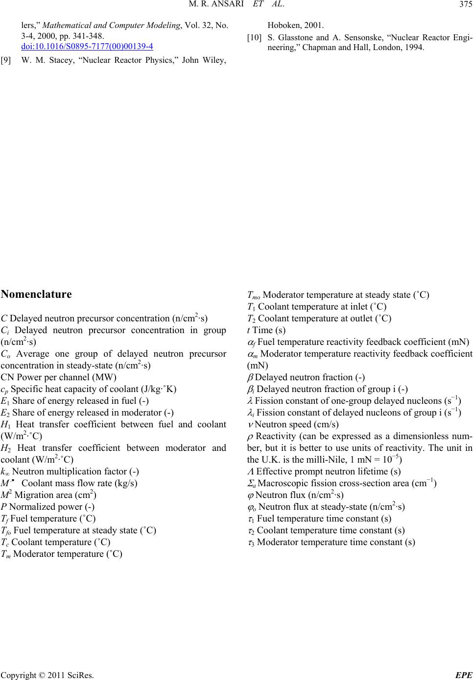
Tra nsient Response to Reactivity Step Disturba nce
T
f
T
c
T
m
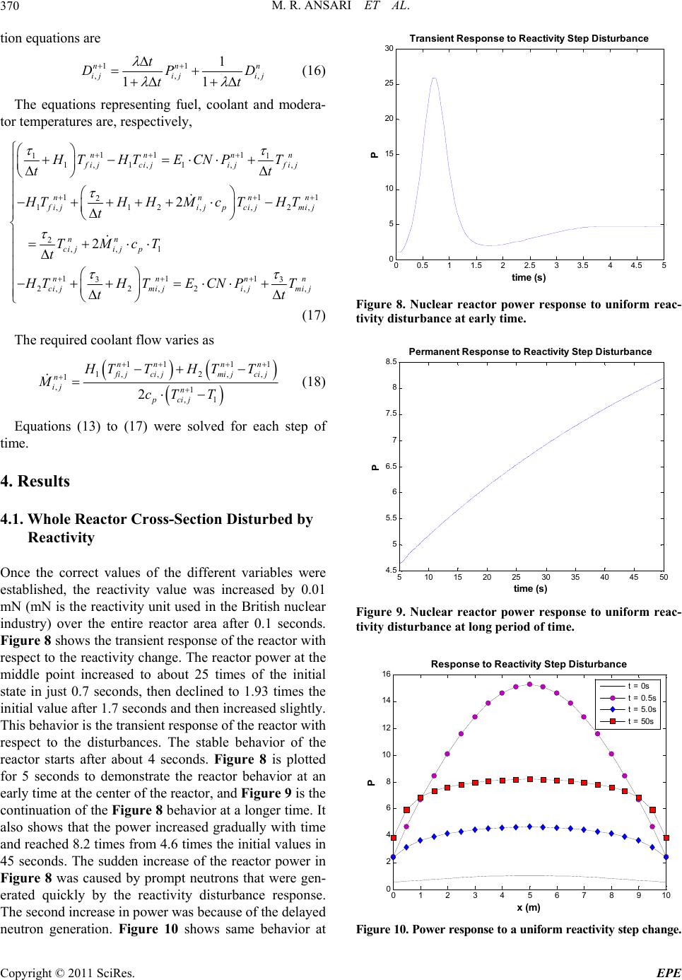
Figure 24. Transient behavior of fuel, coolant and modera
tor to symmetric reactivity disturbance at early time. -
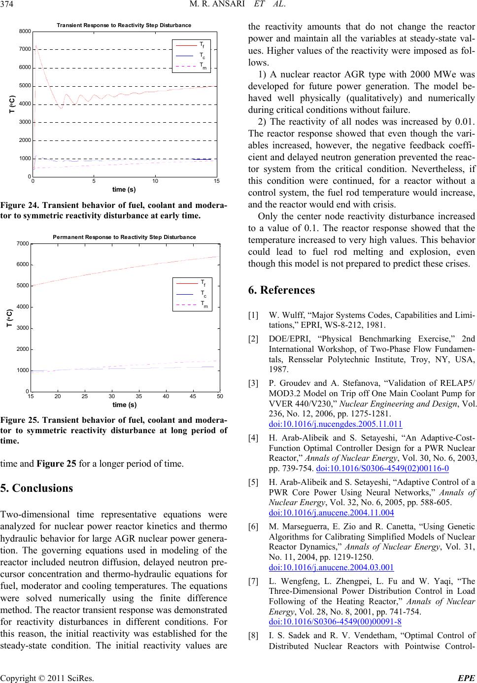
15 20 25 30 35 40 45 50
0
1000
2000
3000
4000
5000
6000
7000
time (s)
T (

C)
Perm anent Response to Re activity Ste p Disturba nce
T
f
T
c
T
m
VVE
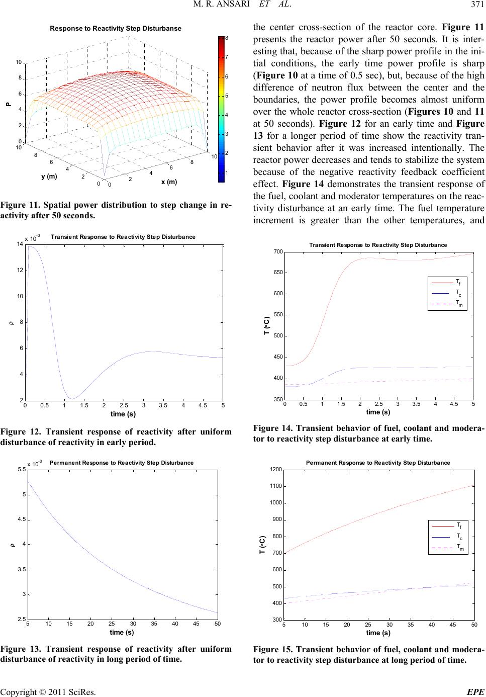
Figure 25. Transient behavior of fuel, coolant and modera
tor to symmetric reactivity disturbance at long period o
nd Figure 25 for a longer period of time.
ime representative equations
ped for future power generation. The model be-
ha
ough the vari-
ab
showed that the
te
jor Systems Codes, Capabilities and Limi-
tations,” EPRI, WS-8-212, 1981.
hase Flow Fundamen-
.2 Model on Trip off One Main Coolant Pump for
-
f
time.
time a
5. Conclusions
wo-dimensional tT
a
were
nalyzed for nuclear power reactor kinetics and thermo
hydraulic behavior for large AGR nuclear power genera-
tion. The governing equations used in modeling of the
reactor included neutron diffusion, delayed neutron pre-
cursor concentration and thermo-hydraulic equations for
fuel, moderator and cooling temperatures. The equations
were solved numerically using the finite difference
method. The reactor transient response was demonstrated
for reactivity disturbances in different conditions. For
this reason, the initial reactivity was established for the
steady-state condition. The initial reactivity values are
the reactivity amounts that do not change the reactor
power and maintain all the variables at steady-state val-
ues. Higher values of the reactivity were imposed as fol-
lows.
1) A nuclear reactor AGR type with 2000 MWe was
develo
ved well physically (qualitatively) and numerically
during critical conditions without failure.
2) The reactivity of all nodes was increased by 0.01.
The reactor response showed that even th
les increased, however, the negative feedback coeffi-
cient and delayed neutron generation prevented the reac-
tor system from the critical condition. Nevertheless, if
this condition were continued, for a reactor without a
control system, the fuel rod temperature would increase,
and the reactor would end with crisis.
Only the center node reactivity disturbance increased
to a value of 0.1. The reactor response
mperature increased to very high values. This behavior
could lead to fuel rod melting and explosion, even
though this model is not prepared to predict these crises.
6. References
[1] W. Wulff, “Ma
[2] DOE/EPRI, “Physical Benchmarking Exercise,” 2nd
International Workshop, of Two-P
tals, Rensselar Polytechnic Institute, Troy, NY, USA,
1987.
[3] P. Groudev and A. Stefanova, “Validation of RELAP5/
MOD3
R 440/V230,” Nuclear Engineering and Design, Vol.
236, No. 12, 2006, pp. 1275-1281.
doi:10.1016/j.nucengdes.2005.11.011
[4] H. Arab-Alibeik and S. Setayeshi, “An Adaptive-Cost-
Function Optimal Controller Design for a PWR Nuclear
Reactor,” Annals of Nuclear Energy, Vol. 30, No. 6, 2003,
pp. 739-754. doi:10.1016/S0306-4549(02)00116-0
[5] H. Arab-Alibeik and S. Setayeshi, “Adaptive Control of a
PWR Core Power Using Neural Networks,” Annals of
Nuclear Energy, Vol. 32, No. 6, 2005, pp. 588-605.
doi:10.1016/j.anucene.2004.11.004
[6] M. Marseguerra, E. Zio and R. Canetta, “Using Gen
Algorithms for Calibrating Simplifie
etic
d Models of Nuclear
Reactor Dynamics,” Annals of Nuclear Energy, Vol. 31,
No. 11, 2004, pp. 1219-1250.
doi:10.1016/j.anucene.2004.03.001
[7] L. Wengfeng, L. Zhengpei, L.
Three-Dimensional Power Distribut
Fu and W. Yaqi, “The
ion Control in Load
Following of the Heating Reactor,” Annals of Nuclear
Energy, Vol. 28, No. 8, 2001, pp. 741-754.
doi:10.1016/S0306-4549(00)00091-8
[8] I. S. Sadek and R. V. Vendetham, “Optima
Distributed Nuclear Reactors with P
l Control of
ointwise Control-

M. R. ANSARI ET AL. 375
lers,” Mathematical and Computer Modeling, Vol. 32, No.
3-4, 2000, pp. 341-348.
doi:10.1016/S0895-7177(00)00139-4
[9] W. M. Stacey, “Nuclear Reactor Phy
sics,” John Wiley,
A. Sensonske, “Nuclear Reactor Engi-
omenclature
Delayed neutron precursor concentration (n/cm2·s)
oup
e one group of delayed neutron precursor
lant (J/kg·˚K)
or (-)
d coolant
ansfer coefficient between moderator and
cation factor (-)
ady state (˚C)
mo Moderator temperature at steady state (˚C)
perature reactivity feedback coefficient (mN)
yed neutron fraction (-)
roup i (-)
cleons (s−1)
ed as a dimensionless num-
a (cm−1)
ate (n/cm2·s)
s)
)
neer
Hoboken, 2001.
[10] S. Glasstone and
ing,” Chapman and Hall, London, 1994.
NT
T1 Coolant temperature at inlet (˚C)
C T2 Coolant temperature at outlet (˚C)
Ci Delayed neutron precursor concentration in grt Time (s)
(n/cm2·s)
Co Averag

f Fuel tem

m Moderator temperature reactivity feedback coefficient
concentration in steady-state (n/cm2·s)
CN Power per channel (MW)
(mN)
 Dela
cp Specific heat capacity of coo 
i Delayed neutron fraction of g
E1 Share of energy released in fuel (-)  Fission constant of one-group delayed nu

i Fission constant of delayed nucleons of group i (s−1) E2 Share of energy released in moderat
H1 Heat transfer coefficient between fuel an  Neutron speed (cm/s)
(W/m2·˚C)
H2 Heat tr
 Reactivity (can be express
ber, but it is better to use units of reactivity. The unit in
the U.K. is the milli-Nile, 1 mN = 10−5)
 Effective prompt neutron lifetime (s)
coolant (W/m2·˚C)
k Neutron multipli
M. Coolant mass flow rate (kg/s) 
a Macroscopic fission cross-section are
M2igration area (cm2) M
 Neutron flux (n/cm2·s)
P Normalized power (-) 
o Neutron flux at steady-st
Tf Fuel temperature (˚C)

1 Fuel temperature time constant (s)
Tfo Fuel temperature at ste 
2 Coolant temperature time constant (
Tc Coolant temperature (˚C) 
3 Moderator temperature time constant (s
Tm Moderator temperature (˚C)