Paper Menu >>
Journal Menu >>
 Advances in Pure Mathematics, 2011, 1, 105-117 doi:10.4236/apm.2011.14023 Published Online July 2011 (http://www.SciRP.org/journal/apm) Copyright © 2011 SciRes. APM Left Eigenvector of a Stochastic Matrix S ylva i n Lavall e ´ e Departement de mathematiques, Universite du Quebec a Montreal, Montreal, Canada E-mail: sylvain.lavallee@uqtr.ca Received January 7, 2011; revised June 7, 2011; accepted June 15, 2011 Abstract We determine the left eigenvector of a stochastic matrix associated to the eigenvalue 1 in the commu- tative and the noncommutative cases. In the commutative case, we see that the eigenvector associated to the eigenvalue 0 is , where is the M 1 (,, ) n NN i Nith principal minor of , where is the identity matrix of dimension . In the noncommutative case, this eigenvector is , where is the sum in of the corresponding labels of nonempty paths starting from and not passing through in the complete directed graph associated to . =n NMI 1 1 (,P i n I n1 ) , n Pi P ij a iM Keywords: Generic Stochastic Noncommutative Matrix, Commutative Matrix, Left Eigenvector Associated To The Eigenvalue 1, Skew Field, Automata 1. Introduction It is well known that 1 is one of the eigenvalue of a stochastic matrix (i.e. the sum of the elements of each row is equal to 1) and its associated right eigenvector is the vector . But, what is the left eigenvector associated to 1? (1,1, ,1)T In the commutative case, this eigenvector is the vector 1 (,, ) n M M , where i M is the i principal minor of the matrix. This formula is known in probability theory; it amounts to finding the stationary distribution of the finite Markov chain whose transition matrix is the stochastic irreducible matrix. th In the noncommutative case, we must involve inverses of elements of the skew field and as these may be undefined, we take a generic noncommutative stochastic matrix: this is the matrix of noncommuting vari- ables ij subject only to the stochastic identities; i.e. the sum of each row equals one. () ij a a We work in the free field generated by these variables (in the sense of Paul Cohn), which we call the stochastic free field. Considering the complete digraph on the set , let i {1,,}n M be the set of paths from to i. Let i be the paths starting from and not passing through again. We identify i with the noncom- mutative power series which is equal to the sum of all the words in i and we still denote this series by i. Next we show that the elements i P i i P P P 1 i P can be evaluated in the stochastic free field and that the vector is fixed by our matrix; moreover, the sum of the 1 1 (,, n PP 1 i P 1 ) is equal to 1, hence they form a kind of noncommutative limiting probability. These results have been proved in [1] but the proof proposed in this paper are completely different. Indeed for the major part the proof in these two instances, we use elementary operations on the rows and the columns of the matrix. 2. Commutative Case The commutative case is well known in probability theory. Indeed, we calculate the limit probability of a finite Markov chain by replacing the stochastic matrix by M MI, where is the identity matrix of the appropriate dimension. For this, we use the Markov chain tree Theorem, where this calculus is expressed in terms of spanning trees. The Markov chain tree theorem gives a formula for the stationary distribution of a finite Markov chain. Equivalently, this formula gives a row vector fixed by a matrix fixing . This theorem is attributed to Kirchoff by Persi Diaconis, who gives a probabilistic proof of it (see [2] p. 443 and 444). See also [3,4]. I (1,1, ,1)T The proof uses only the definition of the determinant which involves the principal minors. Proposition 1 Let be a stochastic matrix and M 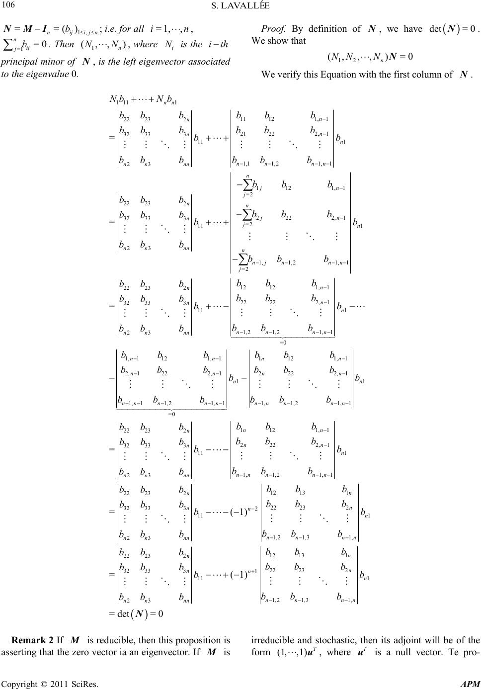 S. LAVALL E ´ E Copyright © 2011 SciRes. APM 106 n1, ==() nijij b NMI n ; i.e. for all , =1,,in =1 =0 ij jb . Then , where is the i 1 (,, ) n NN i Nth principal minor of , is the left eigenvector associated to the eigenvalue 0. N Proof. By definition of , we have N det= 0N. We show that 12 (, ,, )=0 n NN N N We verify this Equation with the first column of . N 1111 11121, 1 22 232 21222, 1 32 333 11 1 1,11,21, 1 23 112 1,1 =2 22 232 222 2,1 32 333 =2 11 23 1, =2 = = nn n n n n n nn nn nn nn n jn j nn jn n j nn nnn nj n j NbN b bb b bb b bb b bb b bb bb b bb b bb b bb b bb b bb b b bb b bb 1 1,21, 1 12121, 1 22 232 22222, 1 32 333 11 1 1,21,21, 1 23 =0 1, 1121,1 2, 1222,1 1, 11,21, 1 =0 = n nn n n n n n nn nn nn nn nn nn nn nnn b b bb b bb b bb b bb b bb bb b bb b bb b bb b bb b 112 1,1 222 2,1 11 1,1,21, 1 112 1,1 22 232 2222,1 32 333 11 1 1,1,21, 1 23 22 232 32 333 11 23 = =(1 nn nn nn nn nnn nn n nn n n nn nnn nn nn n n nn nn bb b bb b bb bb b bb b bb b bb b bb b bb bb b bb b bb b bb b b bb b 12 131 22 232 2 1 1,2 1,31, 12 131 22 232 22 232 32 3331 11 1 1,2 1,31, 23 ) =(1) =det =0 n n n n nn nn n n n nn n nn nn nn nn bbb bb b b bb b bb b bb b bb b bb b bb bb b bb b N Remark 2 If is reducible, then this proposition is asserting that the zero vector ia an eigenvector. If is irreducible and stochastic, then its adjoint will be of the form , where is a null vector. Te pro- M M(1,,1) T uT u  S. LAVALL E ´ E Copyright © 2011 SciRes. APM 107 position follows from the cofactor formula for the adjoint. 3. Noncommutative Case In [1], the authors have prove in two manners that are actually similar, Theorem 9. In the first, results from variable-length prefix codes are required; and the second deals with general variable-length codes, not necessarily prefix. Moreover, in Appendix 2 of [1], we see how the theory of quasideterminants may be used to obtain these results on noncommutative matrices. The major part of the new proof of this Theorem involves only the elementary operations on the rows and on the columns of the stochastic matrix. Therefore, we need the following results. 3.1. Languages and Series Let A be a finite alphabet and * A be the free monoid generated by A . A language is a subset of a free monoid * A . A language is rational if it is obtained from finite languages by the operations (called rational) union, product (concatenation) and star. The product of two languages is 12 LL 12 1122 ,wwwLwL, and the star of is L * 10 =,0= n ni n LwwwLn L . Ra- tional languages may be obtained by using only unam- biguous rational operations; these are: disjoint union, unambiguous product (meaning that if , then has a unique factorization 12 , ii 12 wLL www=wwL ) and the star restricted to languages which are free submonoids of * L * A . A formal series is an element of the -algebra of noncommutative series A , where A is a set of noncommuting variables. A rational series is an element of the smallest subalgebra of A , which contains the -algebra of noncommutative polynomials A , and which is closed under the operation 1 * =0 ==1 n n SS SS which is defined if has zero constant term. We denote by the -algebra of rational series. S rat A Let be a rational language. Since may be obtained by unambiguous rational expressions, it follows L L that its characteristic series wL is ratio- nal. We shall identify a language and its characteristic series. This is exposed in [5] or [6]. wA 3.2. Free Field Let be a field. If the multiplicative group of is commutative, then is a commutative field. Else, is called skew field. The ring of rational formal series in noncommutative variables rat A is not a skew field. However, skew fields containing A do exist. One of them is the free field (in the sense of Cohn), denoted . The free field is the noncommutative analogue of the field of fractions of the ring of commu- tative polynomials. There are several constructions of the free field: Amitsur [7], Bergman [8], Malcolmson [9], Cohn [10] and [11]. A square matrix of order n is full if it can’t expressed as a product of matrices 1nn by . 1nn Theorem 3 ([11], Thm 4.5.8 .) Each full matrix with coefficients in M X is invertible in the free field. A square matrix of order is called ho llow if it contains a n pq block of zeros such that 1pqn . Example 4 The matrix 001 001 111 is hollow since there is a 22 block of 0 and . 4>3 Proposition 5 ([11], Prop. 4.5.4) A hollow matrix is not full. Proposition 6 Take , and 1n nn M 1n , where is a skew field. We suppose that M is invertible. Then 0 M is invertible if and only if 10 M . Proof. () Suppose that , then the inverse 1 = cM 0 of 0 M is 11111 11 1 1 MMcMMc cM c Indeed, this matrix is the right inverse of since M 111111 11 1 1111 1111 1111 11 11 111 1 1111 11 == 0 ()( =() 1 = cc c M 1 ) MMM MMc cM c MMMcMcMM cc MMcM Mc cMcMc c MMcM Mc 10 =01  S. LAVALL E ´ E Copyright © 2011 SciRes. APM 108 This matrix is also the left inverse of since M 111111 11 1 1 111111 111 11 111 1111111 1 = 11 = 0 ()() =() () 1 c c M MMcMMc cM c MMcMMMc MMcM cMMc cM McMcMMc M cM 11 = cc 10 =01 Suppose that ()0 M is invertible. Let M be its inwe have Hence 1 verse. Then 0 = 00 M 1 == 0 M and = 0 0 . It follows that 1 = M 1 == M 1 is proposition, we de follo ry 7 Let 10 M From theduce thwing result. Corolla , M and be with coeffic matrices ients in A where M is full. If 0 M is not full (in paar, if rticul 0 M is by elementary operations on the lines and on the columns to a hollow 3. Let be a generic noncommutative matrix; tive var ld. We equivalent matrix) then in the free field. 1=0 M 3. Generic Stochastic Matrices i.e. the ij a are noncommutaiables. We denote the corresponding free fie associate to M 1, =ij ijn a M the matrix S : it’s exactly the same matrix of which the coefficients satisfy the dentities stochastic i (1) In other words, the sum of each line of =1j =1,, ,=1 n ij ina S is equal to 1; hence S is a stochastic matrix. We call S a gene- ric noncommutative stochastic matrix. The algebra over generated by its coefficients is associative ra, it is isomorph to the algebr algeb free a a since,ai j ij . e stochastic /( 1) ij h by Indeedn eliminate the with t relations We denote thbra , we ca (1). ii a is algea . field called Hence,e is a corresponding free stochastic free field denoted ther S . 3.4. Paths Consider the set of nonempty paths in the complete directed graph with a set of vertices 1,, n starting from i and not passing through i; we denote by i P the sum in ij a of all the corresp tional series, and t of the le onding words. It is defines an element classically a rahus free field . Examp 8 =ab cd M. The graph is then ** 12 =1 ,=1PbdPc a We shall also consider rational expressions over any Ia a ctua nocal embedding of into seen as follows: let tional ace in it the skew field D, and say that such an expression is evaluable in D if it can be evaluated without inversion of 0. f the elements of D appering in the rationl expression lly in a subring R of D, we say that the expression is over R. There is a cani are a rat A ny ra y 1T ser , which can be S be a ies, we reploperation * T b 1 , which is age of ; then evalua one obtains a rational expressi ble in and represents the im on in S under the embedding . Thus, rat A each rational  S. LAVALL E ´ E Copyright © 2011 SciRes. APM 109 language and each rational series is naturally an element of the free field. See [12]. By Theorem 1 of [1], the can be evaluated in the stochastic free field. n now state the main result of this paper. rem 9 Let i P We ca Theo 1, =ij ij n a M be a generic stochastic noncommutative matrix. Let defined as ab i ove. Then 11 11 11 ,,= ,, nn P be P PPP M (2) In other words, 11 1,, n PP is the left eenvector associated to the eigenvalueo ig be the m 1 f M. Example 10 (Continued.) Let be S atrix with =1ab and =1cd. We show that 11 11 12 12 ,=, M P PPP M From this systehe two following equa- m, we deduce t tions: 1 1= 1 Pa P 1 1 (4) n (3), we have (5) * 1 2 = d Since we again obtain Equation (5), it follows that Equation (4) is also satisfied. Proof of Theorem 9. Let be the matrix of the automaton and be the langua starting fr and not passing through . We have ,n where Let 12 1 dP (3) P 12 2 1=aPdP 11 From the Equatio 11 1 12 1 1=Pa PdP 11 21 1=1PdPa ** 21 =dP aP * * 1=1dcaabd ** ** *** * 1= 1daa ad d da *** =daad Hence, Equation (3) is satisfied. From the Equation (4), we have 11 12 1PaPdP 11 12 1=1Pa ** 12 =aP dP 1, =ij ij n a M i P om ge of the labels of the paths i i =1 =,=1,, n iij j PLi =1 =1, 1, = kk kj if ij ==, nn ij ik kjijikkj LLaaLaifi j i S be the system composed of the Equa- tions , in n i P1,1,1 ,, , ,, iiiii LLL L . 1 Multlying to the left by ip i P each equation ofwe obtain the system n i S, 1, 1 : ii ij jji i T Pa 11 1 1, 1=,=1,, n n iij iikkj kki PPLi PLa 1 = ii j PL Let i ij QPL, then we have n 1 = ij 1 1, 1 1, 1=,=1,, : = ii j jji in ijiijik kj kki PQi T QPa Qa n This system transforms into the following system We show that 1 1, 1=,=1,, n iij jji i iijij jj PQin U PaQ aQa 1 : 0= n 1, , 1ikkj kki kj 11 11 =1 n kk k Pa P Define 1 (6) We show that . So Equation (6) is converted into the following Equation 0 (7) ua- tion (7) and the systems . We have the matrical representation 1 1 =kk k RPa 1 =1 n P =0R 11 1111 =2 1= n kk k RP aPa Consider the system of the 21n Equations: Eq n 1,,UU n 11 11213 1221232 1 1,1 ,,,,,,,,,, ,,, = nn nn nn RP QQQP QQQ PQ Q Eλ ,  S. LAVALL E ´ E Copyright © 2011 SciRes. APM 110 12 aa ,1 ,1 11121, 11, 11 21222, 12, 12 1,11,21, 11, 11, 1,11,21, 11,11, ,1,2, 1, 1 1 1 =1 1 1 mmmm mmmn mm mm m m mmmmmmn mmmmmmmn nnnm nmnn a aa aaa aa aaa aa aa aaa aaa aa aaa aa n n A E where =1, ,mn and =(0, ,0,1, ,1) ntimes . is a square mder atrix of or21n. We have 1 =, RE 2 0,,0) T n times and =(1, =0 E F . The orde this r of matrix is . Moreover, with the stochastic identities, we have 22n i B where the are defined by n n n a 12,1 ,1 1121,11,11 =1,1 2122, 12,12 =1, 2 1,11,1,11, =1,2, 1 1,11,21, 11,1, =1, 1 ,1 ,2 mmmm mmmn n kmm kk n km m kk n mmkmm m kk km n mmmmmk mn kkm nn aaa aa aaa aa aaa a aaa a a a aa ,1 ,1 =1, n nm nmnk kkn aa 1, 2 = mm a a B aa a  S. LAVALL E ´ E Copyright © 2011 SciRes. APM 111 To show that , we show that the matrix =0R F is hollow. For this, we apply elementary operations on the rows and on thns ofe colum F Step 2. We want a until F coa ntains s t block of 0 s uch that2 n3st . Step 1. We eliminate the first rowe and the last column of F . We obtain the square matrix 1 F of order ). 21n (22nst nn block of 0 in the right upper corner of 1 F . For this, we consider the row of j-th 1 F (corresnding t- row ). By structio , the first index of the elements of the ro t weer the first c. oeth the ve blocks po n of w of its ele tion of h ha o the block is ents is We repeat rst index e j j block j th . Now, 2 B . Such a this quals to of c such that this ratio j in B onsi row exists by n w the 1 d i con j- row co 3 1 B his which passes in the m 2 B the fi th index of nstru row whic ,, p n BB w of . We add each one of these rows to the j-th ro 1 F . It follows that the atrix n ar last ele e all equal to we subtract the last row ments of the 1. From j each 1 first rows of this new m j row of the first rows, of F . We obtain the following matrix where 1,11 1 2, 12, 12 m mn m n a a aaa 112 1, =1,1 21 2 =1, 2 ,1,2,, 1,1 =1, = n k kk n km kk m n nn nmnm kkn aa a aa aa aa C nk a . We reduce =2,, mn 2 F 3 in removing the last line column if we start from the end. We atrix and the have the nth following m F of order 2 n, (1 s tn ). Step 3. Consider the rows of i L3 F , where and . We want thathe last mews to be e to >in ele- nm 0modin nts of these ro t quals (1) t n 0. Le=ik , ation wher , then n e mn01we apply the transform (1) (1) = iknknmk LLL L , to obtain the matrix =2,,mn where, for all , 1, =,=,= mm mijmijij ijnj ijn dbd mm bb DB (1)n We remove the rows where and i L>in ni and the (1n) last columns of 4 F to obtain the matrix 5 F of order (st 2 n2n ).  S. LAVALL E ´ E Copyright © 2011 SciRes. APM 112 where m D is the matrix obtained from m D in remo- Step 4. Denote by the first column of the matrix and byn of ving the last row. 1 m C the colum m C m d 5 F , which is the ex- tension of . We to be transformed into a of. For this, we apply the 1 m , C 0 want , ,mn 1 m C vector op =2 eration 23 j n dcc c, where is the it i ch colum 3 n of F . Finally we want that the first n elements t column of th of e firs 5 F to transformati be all 0; for this, we apply the on 12 cc c n. We obtain the matrix 6 F of order ) 21 (stnn22nn where m C is the mtrix obtaained from by remfirst column. Step 5. We want each will be transformed into a m colum m C oving the m C atrix of 0. To each n q of m , denoted m C q C correspo ding to the ,*,,* T q n column = qm d C of 6 F . By construction of (hence of ), there exists a column of m Cm C q b6 F such that * =,*,, T q qm b C. Hence, for all, we calculate . We obtain the matrix qqq db 7 F of). order 21nn (22nnst Step 6. Permuting tst and the nth column of 7 he fir F , we x 8 obtain the matri F of der 2 nor 1n (22stnn ). where 1 B is the 1 B block obtained from by removing . We find a 1block of 0 upper corn the first column located in the right 2 11nn 2 )(1nn er and 22 8 = 21=dimnn nn F It follows that F is a hollow. From Corollary 7, Let 1 is Example 11. 11 1 =1 == =0 n kk kPa P RE . Hence 11 ,,P 11n P the left eigenvector associated to 1. 11 1213 aa 21 a 22 23 31 3233 = a aa a aa M be a generic in w s non de commutative matrix hich the variables satisfy the stochastic intitie123ii i aa a=1 e associate theutomn , =1,2,3i. W at ao Let 1 P be the language recognized by automaton the Let ij L be the language of start from i to j. We have 1111213 =,PL LL words which where 11 =1L  S. LAVALL E ´ E Copyright © 2011 SciRes. APM 113 stem each equation of 1212 1222 1332 =LaLaLa 1313 12231333 =LaLaLa We have the sy 12 13 := SL aLaL 112 1212221332 1313 1223 13 1 = PLL a LaLaLa 33 Multiplying to left by 1 P 1 S1 , we obtain the system Define , then We obtain a Permuting the index of the equations of , we obtain the two following systems a a To show that 1 U 1 22123 1 2121123 31 22321132333 1= :0= 1 0= 1 PQQ UPaQaQ PaQaQ a 2 21 1 1 33132 1 3331311132 21 1 33231123222 1= :0= 1 0= 1 PQQ UPaQaQ PaQaQ a 11 1 1 11 11 121 1= := PPLPL TPLP 1 12113 1 1 121122211332 111 1 1 13113112231 1333 = aPLaPLa PLPa PLaPLa 111111 123 123 ,,= ,,PPP PPP M 111 , it suffices to prove that 1 111221 3311 =Pa Pa PaP . Define 1 1 1 = ij ij QPL 111 111221331 1 =RPa PaPa P then 1 11213 1 112 112 1222 1332 1 1311312231333 1= := = PQQ TQPa QaQa QPaQaQa 111 111221331 1=RPaPa Pa 0 Under the matrical system, we have 11 112 13221 23331 32 ,1,,,,,,,, =RPQQP QQP QQ Eλ 1 11213 1 1112122213 32 1= :0= 1 PQQ UPaQa where Q = 0,0,0,0,0,0,0,1,1,1λ 1 1 1312231333 0= 1PaQaQ a and 0 0 0 0 0 0 0 1 1 1 a We have 11 1213 22 23 32 33 2121 23 11 13 31 33 3131 32 11 12 21 22 100000000 1 000010 0 1000010 0 1000010 00 0001 =000 10001 000 10001 0000 00 00000 100 00 100 aa a aa aa aaa aa aa aa aa aa E 000 1 = RE , ,0,0,0,0,0,0,0 where and E with stochastic iden- tities equal to 0 0 0 0 0 0 0 1 1 1 a = 1,0,0T 1 12 13 12 13 21 2323 3231 32 2121 23 13 3131 32 3131 32 12 1312 2121 23 00000000 000010 0 000010 0 000010 00 0001 0 001 0000 001 0000 00 00000 00 00000 00 aa aa aa a aaa aaa aa a aaa aa aa a aaa 12 13 00 0 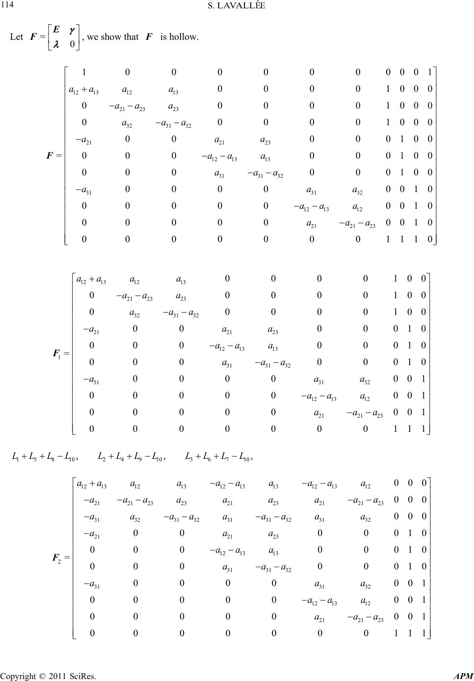 S. LAVALL E ´ E Copyright © 2011 SciRes. APM 114 Let =0 E F , we show that F is hollow. 1 0 0 0 0 0 0 0 0 0 a 0 0 0 0 0 0 1 1 1 a , 000 0 0 0 1 aa aaaa aaa a a 1 1 12 131213 21 2323 323132 2121 23 13 3131 32 3131 32 12 1312 2121 23 1000000000 0 0 0 0000100 0 0000100 00 00010 00 00 0010 0 00 0010 0000 001 00000001 00000001 0000000111 aa aa aa a aaa aaa aa aaa aa aaa aaa F 0 00010 a 12 13 = 0 12 131213 21 2323 323132 2121 23 12 13 1 3131 32 3131 32 12 1312 2121 23 000010 0 000010 0 000010 00 0001 00 00 001 =00 001 0000001 000 0 000 000 0 000 000000011 aa aa aa a aaa aaa aa a aa aa aa a aaa F 13 00a 15810 2491036710 ,,LLLL LLLL LLLL 12 13121312 131312 1312 2121 232321232121 23 313231 323131 323132 21 23 12 1313 2 3131 32 3131 32 12 1312 000 000 0001 00 00 001 =00 00 001 0000 00 000000 aaaa aaaaa aaaaaaaa a aa aaa aaa aa aaa F 2121 23 01 0000000 000000011 aaa 21 00a 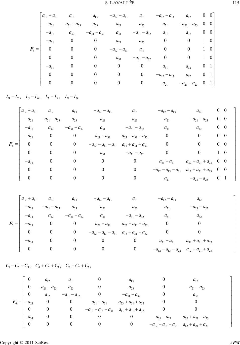 S. LAVALL E ´ E Copyright © 2011 SciRes. APM 115 0 0 1 1 a , a aaa , aaa 1213 12131213131213 12 2121232321232121 23 313231 323131323132 2121 23 3121313 3131 32 3131 32 12 1312 00 00 00 00 001 =00000 10 00 00 01 0000 0 00 0 0 00 00 0 0 0 aa aaaaaaa a aaaaaaaaa aaaaaaaa a aaa aaa aaa aa aaa a F 212123 01aa 46 56 79 89 ,,,LLLL LLLL 12 13121312 131312 1312 2121 232321232121 23 313231 323131 323132 2121 31233132 4 121331133132 3131 32 3131 21 00 00 00 000 000 =00000 00 00 00010 00 00 aa aaaaaaaa aaaa aaa aa aaaa aaaaa aaaaaa aaaaaa aaa aaa F 3221 23 12 1321122123 2121 23 00 00 00000 00 00001 aa aaaaaa aaa 12 13121312 131312 1312 2121232321232121 23 313231 323131 323132 521 2131233132 12 13 3113 3132 3131 213221 23 12 1321 =0000 00 000 00 00 00 000 aa aaaaaaaa aaaaaaaaa aaaa aaaaa aaaaaa aaaaaa aaa aaaa F 1221 23 aa 123 423 623 ,,CCCCCCCCC 12 131312 21 23232321 23 32313231 3232 6212131233132 12 13 31133132 3131 213221 23 12 1321122123 000 000 000 =000 0 00 000 00 00 00 000 aa aa aa aaaa aaaaaa aaaaaa aaaaaa aaa aaaaaa F  S. LAVALL E ´ E Copyright © 2011 SciRes. APM 116 aaa a We have a block of zero with . It follows that 53 72 ,,CC CC 12 13 21 2323 323132 7212131 233132 1213 31 13 31 32 3131 213221 23 12 1321122123 00000 00000 00000 =000 0 00 000 00 00 00 000 aa aa a aaa aaaaaa aaaaaa aaa aaaaaa F 13 CC 13 12 2321 23 31 3232 8 212131233132 12 13 31133132 3131 213221 23 12 1321122123 00000 00000 00000 =0 000 0000 0 0000 0000 0 aa aaa aa a aaaaaa aaaaaa aaaaa aaaaaa F 35 8>7 F Pa This pr is hollow. By C 11 221 Pa allo orollary 7, 0 . Theorem 12. Let be defined as above, then in we have (8) Proof. Define 1 1 1113311 ==PaP R oof ws us to prove the next result. i P 1 =1 =1 n i i P 1 =1 =1 n i i P R we will show that We replace the first column of the matrix 1 =1 =1 n i i P R E by the vector and the first element of by 1. Denoted 1,1,0, ,0,1,0, ,0, ,1,0, ,0T λ E and λ these two matrices. Consider the matrix =0 E F . We repeat each step of the proof of Theorem 9, except for the last operation of step 4, which concerns the first column. Again, we show that F =0. is hollow, and hence, by Corollary 7, we have This proves Equation (8). Example 13. (Continued.) R 11 11* 1211 11* 1*1 11 111 =1byEquation(5) ==1= PP PPad PPbdPbd PP =1 4. Conclusions One of the contribution of this article is the using of elementary operations on the lines and the columns. This method provides a new way to obtain some results in skew field theory with a minimum of knowledge of this theory. Moreover, Theorems 9 and 12 are proved exactly the same way. 5. Acknowledgements I am obliged to thank to Christophe Reutenauer for his comments, corrections and suggestions. 6. References [1] S. Lavall´ee, D. Perrin, C. Reutenauer and V. Retakh, “Codes and Noncommutative Stochastic Matrices,” To  S. LAVALL E ´ E Copyright © 2011 SciRes. APM 117 appear, 2008. [2] A. Broder, “Generating Random Spanning Trees. Proc 30th IEEE Symp,” Proceedings of the 30th IEEE Sympo- sium on Foundation of Computer Science, Boston, 1989, pp. 442-447. [3] V. Anantharam and P. Tsoucas, “A Proof of the Markov Chain Tree Theorem,” Statistic and Probability Letters, Vol. 8, No. 2, 1989, pp. 189-192. [4] D.-J. Aldous, “The Randow Walk Construction of Uni- form Spanning Trees and Uniform Labelled Trees,” SIAM Journal on Discrete Mathematics, Vol. 3, No. 4, 1990, pp. 450-465. [5] J. Berstel and C. Reutenauer, “Les S´eries Rationnelles et Leurs Langages,” Masson, Paris, 1984. [6] J. Bersl and C. Reutenauer, “Rational Series and Their Languages,” 2008. http://www-igm.univ-mlv.fr/~berstel/LivreSeries/LivreSe ries08janvier2008.pdf. [7] A. Amitsur, “Rational Identities and Applications to Al- gebra and Geometry,” Journal of Algebra, Vol. 3, 1966, pp. 304-359. [8] G. M. Bergman, “Skew Field of Noncommutative Ra- tional Functions, after Amitsur,” S´eminaire Schu¨tzen- berger-Lentin-Nivat, Vol. 16, 1970. [9] P. Malcolmson, “A Prime Matrix Ideal Yields a Skew Field,” Journal of the London Mathematical Society, l. 18, 1978, pp. 221-233. [10] P. M. Cohn, “Free Rings and Their Relations,” Academic Press, Salt Lake City, 1971. [11] P. M. Cohn, “Skew Fields: Theory of General Division Rings,” Encyclopedia of Mathematics and Its Applica- tions, Cambridge University Press, Cambridge, 1995. [12] M. Fliess, “Sur le Plongement de l’alg`ebre des S´eries Rationelles non Commutatives dans un Corps Gauche,” Proceedings of the National Academy of Sciences, Paris, 1970. te Vo |