Vol.3, No.7, 600-616 (2011) Natural Science
http://dx.doi.org/10.4236/ns.2011.37083
The wave-corpuscle properties of microscopic particles
in the nonlinear quantum-mechanical systems
Xiaofeng Pang
Institute of Life Science and Technology, University of Electronic Science and Technology of China, Chengdu 610054, China and
International Centre for Materials Physics, Chinese Academy of Science, Shenyang, China;
*Corresponding Author:
Received 12 December, 2010; revised 20 February, 2011; accepted 3 March 2011.
ABSTRACT
We debate first the properties of quantum me-
chanics and its difficulties and the reasons re-
sulting in these diffuculties and its direction of
development. The fundamental principles of
nonlinear quantum mechanics are proposed
and established based on these shortcomings
of quantum mechanics and real motions and
interactions of microscopic particles and
backgound field in physical systems. Subse-
quently, the motion laws and wave-corpuscle
duality of microscopic particles described by
nonlinear Schrödinger equation are studied
completely in detail using these elementary
principles and theories. Concretely speaking,
we investigate the wave-particle duality of the
solution of the nonlinear Schrödinger equation,
the mechanism and rules of particle collision
and the uncertainty relation of particle’s mo-
mentum and position, and so on. We obtained
that the microscopic particles obey the classical
rules of collision of motion and satisfy the
minimum uncertainty relation of position and
momentum, etc. From these studies we see
clearly that the moved rules and features of mi-
croscopic particle in nonlinear quantum me-
chanics is different from those in linear quan-
tum mechanics. Therefore, nolinear quantum
mechanics is a necessary result of development
of quantum mechanics and represents correctly
the properties of microscopic particles in
nonlinear systems, which can solve difficulties
and problems disputed for about a century by
scientists in linear quantum mechanics field.
Keyw ords: Microscopic Particle; Nonlinear
Interaction; Quantum Mechanics; Nonlinear
Schrödinger Equation; Basic Principle; Nonlinear
Theory; Wave-Particle Duality; Motion Rule
1. INTRODUCTION, WAVE FEATURE OF
MICROSCOPIC PARTICLES AND
DIFFICULTIES OF QUANTUM
MECHANICS
It is well known that several great scientists, such as
Bohr, Born, Schrödinger and Heisenberg, etc. estab-
lished quantum mechanics in the early 1900s [1-9],
which is the foundation and pillar of modern science and
provides an unique way of describing the properties and
rules of motion of microscopic particles (MIP) in mi-
croscopic systems. The elementary hypotheses of quan-
tum mechanics can be described as Eq.1. The states of
microscopic particles is described by a wave func-
tion


,t  r or wave-vector,

,t  r, which represents
the state of the particle at position rand time t and sat-
isfies the following superposition principle:






112 2
,,,tc tct   rrr
or 112 2
CC

 
(1)
where 1

or 1

and 2

or 2

are two states of the
microscopic particle, C1 and C2 are constants relating to
its states of a microscopic particle. The superposition
principle manifests that the linear superposition of two
different states of the particle describes still it’s a state.
Therefore, it is referred to as the linear superposition
principle of states of the microscopic particle. The
changed rules of the state of microscopic particle with
varying of time and space satisfy the following Schrö-
dinger equation:

2
2,
2
iVt
tm



 
r

 (2)
where 22 2m is the kinetic energy operator,


,Vtr is the externally applied potential operator, m is
the mass of particles, In this theory the Hamiltonian op-
erator of the system corresponding dynamic Eq.2 is


22
ˆ2,
H
tmVt r (3)
(2) The mechanical quantity, which denotes the prop-
erties of microscopic particle, is represented by an op-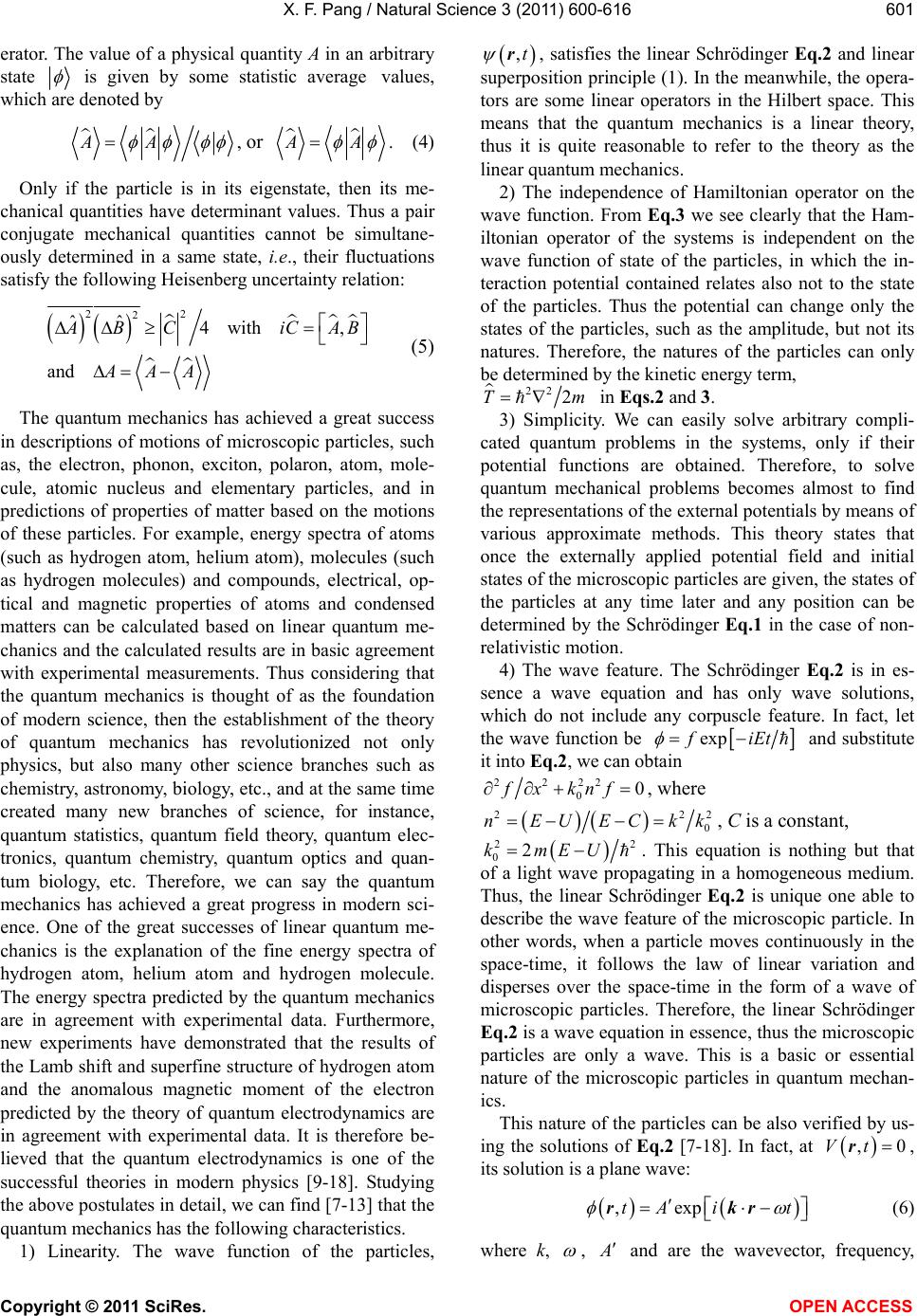

X. F. Pang / Natural Science 3 (2011) 600-616 601
erator. The value of a physical quantity A in an arbitrary
state

is given by some statistic averagevalues,
which are denoted by


AA

 , or


AA

 . (4)
Only if the particle is in its eigenstate, then its me-
chanical quantities have determinant values. Thus a pair
conjugate mechanical quantities cannot be simultane-
ously determined in a same state, i.e., their fluctuations
satisfy the following Heisenberg uncertainty relation:


  

2 22
ˆˆ4 with,
and
AB CiCAB
AAA

 

 
(5)
The quantum mechanics has achieved a great success
in descriptions of motions of microscopic particles, such
as, the electron, phonon, exciton, polaron, atom, mole-
cule, atomic nucleus and elementary particles, and in
predictions of properties of matter based on the motions
of these particles. For example, energy spectra of atoms
(such as hydrogen atom, helium atom), molecules (such
as hydrogen molecules) and compounds, electrical, op-
tical and magnetic properties of atoms and condensed
matters can be calculated based on linear quantum me-
chanics and the calculated results are in basic agreement
with experimental measurements. Thus considering that
the quantum mechanics is thought of as the foundation
of modern science, then the establishment of the theory
of quantum mechanics has revolutionized not only
physics, but also many other science branches such as
chemistry, astronomy, biology, etc., and at the same time
created many new branches of science, for instance,
quantum statistics, quantum field theory, quantum elec-
tronics, quantum chemistry, quantum optics and quan-
tum biology, etc. Therefore, we can say the quantum
mechanics has achieved a great progress in modern sci-
ence. One of the great successes of linear quantum me-
chanics is the explanation of the fine energy spectra of
hydrogen atom, helium atom and hydrogen molecule.
The energy spectra predicted by the quantum mechanics
are in agreement with experimental data. Furthermore,
new experiments have demonstrated that the results of
the Lamb shift and superfine structure of hydrogen atom
and the anomalous magnetic moment of the electron
predicted by the theory of quantum electrodynamics are
in agreement with experimental data. It is therefore be-
lieved that the quantum electrodynamics is one of the
successful theories in modern physics [9-18]. Studying
the above postulates in detail, we can find [7-13] that the
quantum mechanics has the following characteristics.
1) Linearity. The wave function of the particles,


,t  r, satisfies the linear Schrödinger Eq.2 and linear
superposition principle (1). In the meanwhile, the opera-
tors are some linear operators in the Hilbert space. This
means that the quantum mechanics is a linear theory,
thus it is quite reasonable to refer to the theory as the
linear quantum mechanics.
2) The independence of Hamiltonian operator on the
wave function. From Eq.3 we see clearly that the Ham-
iltonian operator of the systems is independent on the
wave function of state of the particles, in which the in-
teraction potential contained relates also not to the state
of the particles. Thus the potential can change only the
states of the particles, such as the amplitude, but not its
natures. Therefore, the natures of the particles can only
be determined by the kinetic energy term,

22
2Tm in Eqs.2 and 3.
3) Simplicity. We can easily solve arbitrary compli-
cated quantum problems in the systems, only if their
potential functions are obtained. Therefore, to solve
quantum mechanical problems becomes almost to find
the representations of the external potentials by means of
various approximate methods. This theory states that
once the externally applied potential field and initial
states of the microscopic particles are given, the states of
the particles at any time later and any position can be
determined by the Schrödinger Eq.1 in the case of non-
relativistic motion.
4) The wave feature. The Schrödinger Eq.2 is in es-
sence a wave equation and has only wave solutions,
which do not include any corpuscle feature. In fact, let
the wave function be


exp
f
iEt   and substitute
it into Eq.2, we can obtain
2222
00fx knf

 , where




222
0
nEUECkk , C is a constant,


22
02kmEU. This equation is nothing but that
of a light wave propagating in a homogeneous medium.
Thus, the linear Schrödinger Eq.2 is unique one able to
describe the wave feature of the microscopic particle. In
other words, when a particle moves continuously in the
space-time, it follows the law of linear variation and
disperses over the space-time in the form of a wave of
microscopic particles. Therefore, the linear Schrödinger
Eq.2 is a wave equation in essence, thus the microscopic
particles are only a wave. This is a basic or essential
nature of the microscopic particles in quantum mechan-
ics.
This nature of the particles can be also verified by us-
ing the solutions of Eq.2 [7-18]. In fact, at


,0Vt

r,
its solution is a plane wave:


,exptA it 

 

rkr (6)
where k,

,
A

and are the wavevector, frequency,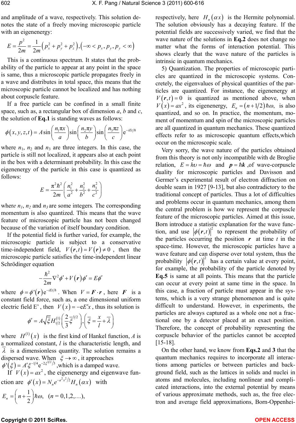

X. F. Pang / Natural Science 3 (2011) 600-616 602
and amplitude of a wave, respectively. This solution de-
notes the state of a freely moving microscopic particle
with an eigenenergy:


2
222
1,,,
22xyz xyy
p
Epppppp
mm

This is a continuous spectrum. It states that the prob-
ability of the particle to appear at any point in the space
is same, thus a microscopic particle propagates freely in
a wave and distributes in total space, this means that the
microscopic particle cannot be localized and has nothing
about corpuscle feature.
If a free particle can be confined in a small finite
space, such as, a rectangular box of dimension a, b and c,
the solution of Eq.1 is standing waves as follows:

3 12 π
ππ
,,, sinsinsine
iEt
nz
nxn y
xyztAabc


 


 

where n1, n2 and n3 are three integers. In this case, the
particle is still not localized, it appears also at each point
in the box with a determinant probability. In this case the
eigenenergy of the particle in this case is quantized as
follows:
2 22 22
3 12
222
π
2
n nn
Emabc





where n1, n2 and n3 are some integers. The corresponding
momentum is also quantized. This means that the wave
feature of microscopic particle has not been changed
because of the variation of itself boundary condition.
If the potential field is further varied, for example, the
microscopic particle is subject to a conservative
time-independent field,  
,0VtVrr, then the
microscopic particle satisfies the time-independent linear
Schrödinger equation

2
2
2VE m



  r

where

'e
iEt


r. When VFr, here
F
is a
constant field force, such as, a one dimensional uniform
electric field E’ , then

eVx Ex

 , thus its solution is

32
1
12
2,
3
x
AH l


 

 
 
where


1
H
x is the first kind of Hankel function, A is
a normalized constant, l is the characteristic length, and

is a dimensionless quantity. The solution remains a
dispersed wave. When

, it approaches

32
14 23
'eA

 


,which is a damped wave.
If

2
Vx ax, the eigenenergy and eigenwave fun-
ction are
 
222ax
nn
x
NeH x



 with
1,
2
n
En





 (n = 0,1,2,…),
respectively, here


n
H
x

is the Hermite polynomial.
The solution obviously has a decaying feature. If the
potential fields are successively varied, we find that the
wave nature of the solutions in Eq.2 does not change no
matter what the forms of interaction potential. This
shows clearly that the wave nature of the particles is
intrinsic in quantum mechanics.
5) Quantization. The properties of microscopic parti-
cles are quantized in the microscopic systems. Con-
cretely, the eigenvalues of physical quantities of the par-
ticles are quantized. For instance, the eigenenergy at


,0Vt

r is quantized as mentioned above, when


2
Vx ax, its eigenenergy,


12 ,
n
En

  is also
quantized, and so on. In practice, the momentum, mo-
ment of momentum and spin of the microscopic particles
are all quantized in quantum mechanics. These quantized
effects refer to as microscopic quantum effects,which
occur on the microscopic scale.
Very sorry, the wave nature of the particles obtained
from this theory is not only incompatible with de Broglie
relation, Eh



 and pk,of wave-corpuscle
duality for microscopic particles and Davisson and
Germer’s experimental result of electron diffraction on
double seam in 1927 [9-13], but also contradictory to the
traditional concept of particles. Thus a lot of difficulties
and problems occur in quantum mechanics, among them
the central problem is how we represent the corpuscle
feature of the microscopic particles. Aimed at this issue,
Born introduce a statistic explanation for the wave func-
tion, and use

2
,t  r to represent the probability of
the particles occurring the position r at time t in the
space-time. However, the microscopic particles have a
wave feature and can disperse over total system, thus the
probability

2
,t  r has a certain value at every point,
for example, the probability of the particle denoted by
Eq.5 is same at all points. This means that the particle
can occur at every point at same time in the space. In
this case, a fraction of particle must appear in the sys-
tems, which is a very strange phenomenon and is quite
difficult to understand. However, in experiments, the
particles are always captured as a whole one not a frac-
tional one by a detector placed at an exact position.
Therefore, the concept of probability representing the
corpuscle behavior of the particles cannot be accepted
[15-18].
On the other hand, we know from Eqs.2 and 3 that the
quantum mechanics requires to incorporate all interac-
tions among particles or between particles and back-
ground field, such as the lattices in solids and nuclei in
atoms and molecules, including nonlinear and compli-
cated interactions, into the external potential by means
of various approximate methods, such as, the free elec-
tron and average field approximations, Born-Oppenhei-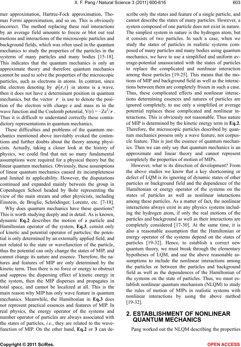

X. F. Pang / Natural Science 3 (2011) 600-616 603
mer approximation, Hartree-Fock approximation, Tho-
mas Fermi approximation, and so on. This is obviously
incorrect. The method replacing these real interactions
by an average field amounts to freeze or blot out real
motions and interactions of the microscopic particles and
background fields, which was often used in the quantum
mechanics to study the properties of the particles in the
systems of many particles and many bodies [15-18].
This indicates that the quantum mechanics is only an
approximate theory and therefore quantum mechanics
cannot be used to solve the properties of the microscopic
particles, such as electrons in atoms. In contrast, since
the electron denoting by

,t  r in atoms is a wave,
then it does not have a determinant position in quantum
mechanics, but the vector r is use to denote the posi-
tion of the electron with charge e and mass m in the
wave function and the Coulemb potential, V(r) = –Ze2/r.
Thus it is difficult to understand correctly these contra-
dictory representations in quantum mechanics.
These difficulties and problems of the quantum me-
chanics mentioned above inevitably evoked the conten-
tions and further doubts about the theory among physi-
cists. Actually, taking a closer look at the history of
physics, we could find that not so many fundamental
assumptions were required for a physical theory but the
linear quantum mechanics. Obviously, these assumptions
of linear quantum mechanics caused its incompleteness
and limited its applicability. However, the disputations
continued and expanded mainly between the group in
Copenhagen School headed by Bohr representing the
view of the main stream and other physicists, including
Einstein, de Broglie, Schrödinger, Lorentz, etc. [7-18].
Why does quantum mechanics have these questions?
This is worth studying deeply and in detail. As is known,
dynamic Eq.2 describes the motion of a particle and
Hamiltonian operator of the system, Eq.3, consist only
of kinetic and potential operator of particles; the poten-
tial is only determined by an externally applied field, and
not related to the state or wavefunction of the particle,
thus the potential can only change the states of MIP, and
cannot change its nature and essence. Therefore, the na-
tures and features of MIP are only determined by the
kinetic term. Thus there is no force or energy to obstruct
and suppress the dispersing effect of kinetic energy in
the system, then the MIP disperses and propagates in
total space, and cannot be localized at all. This is the
main reason why MIP has only wave feature in quantum
mechanics. Meanwhile, the Hamiltonian in Eq.3 does
not represent practical essences and features of MIP. In
real physics, the energy operator of the systems and
number operator of particles are always associated with
the states of particles, i.e., they are related to the wave-
function of MIP. On the other hand, Eq.2 or 3 can de-
scribe only the states and feature of a single particle, and
cannot describe the states of many particles. However, a
system composed of one particle does not exist in nature.
The simplest system in nature is the hydrogen atom, but
it consists of two particles. In such a case, when we
study the states of particles in realistic systems com-
posed of many particles and many bodies using quantum
mechanics, we have to use a simplified and uniform av-
erage-potential unassociated with the states of particles
to replace the complicated and nonlinear interaction
among these particles [19-25]. This means that the mo-
tions of MIP and background field as well as the interac-
tions between them are completely frozen in such a case.
Thus, these complicated effects and nonlinear interac-
tions determining essences and natures of particles are
ignored completely, to use only a simplified or average
potential replaces these complicated and nonlinear in-
teractions. This is obviously not reasonable. Thus nature
of MIP is determined by the kinetic energy term in Eq.2.
Therefore, the microscopic particles described by quan-
tum mechanics possess only a wave feature, not corpus-
cle feature. This is just the essence of quantum mechan-
ics. Then we can only say that quantum mechanics is an
approximate and linear theory and cannot represent
completely the properties of motion of MIPs.
However, what is its direction of development? From
the above studies we know that a key shortcoming or
defect of LQM is its ignoring of dynamic states of other
particles or background field and the dependence of the
Hamiltonian or energy operator of the systems on the
states of particles as well as nonlinear interactions
among these particles. As a matter of fact, the nonlinear
interactions always exist in any physics systems includ-
ing the hydrogen atom, if only the real motions of the
particles and background as well as their interactions are
completely considered [17-30]. At the same time, it is
also a reasonable assumption that the Hamiltonian or
energy operator of the systems depend on the states of
particles [19-32]. Hence, to establish a correct new
quantum theory, we must break through the elementary
hypotheses of LQM, and use the above reasonable as-
sumptions to include the nonlinear interactions among
the particles or between the particles and background
field as well as the dependences of the Hamiltonian of
the systems on the state of particles. Thus, we must es-
tablish nonlinear quantum mechanism (NLQM) to study
the rules of motion of MIPs in realistic systems with
nonlinear interactions by using the above method
[19-32].
2. ESTABLISHMENT OF NONLINEAR
QUANTUM MECHANICS
Pang worked out the NLQM describing the properties

X. F. Pang / Natural Science 3 (2011) 600-616 604
of motion of MIPs in nonlinear systems [17-30]. The
elementary principles, theory, calculated rules and ap-
plications of NLQM are proposed and established based
on the relations among the nonlinear interaction and
soliton motions and macroscopic quantum effect through
incorporating modern theories of superconductors, su-
perfluids and solitons [23-27]. In these physical systems
the Hamiltonian, free energy or Lagrangian functions of
the systems are all nonlinear functions of the wave func-
tion of the microscopic particles which break down the
hypotheses for the independence of the Hamiltonian of
the systems on the states of the particles and the linearity
of the theory in the LQM, the dynamic equations of
microscopic particles, such as superconductive electrons
and superfluid heliem atoms which were depicted by a
macroscopic wave function,


,
,,e
it
tt

 r rr , are
the time-independent and time-dependent Ginzburg-Lan-
dau equations (G-L) and Gross-Pitaerskii (G-P) equation
[33-38], which are in essence the nonlinear Schrödinger
equation and have a soliton solution with a
wave-corpuscle duality because the nonlinear interac-
tions can balance and suppress the dispersive effect of
the kinetic energy in these dynamic equations [23-27].
Therefore, the investigations of essences and properties
of macroscopic quantum mechanics, superconductivity
and superfluid provide direction for establishing nonlin-
ear quantum mechanics [23-27].
Based on the above discussions, the fundamental
principles of nonlinear quantum mechanics (NLQM)
proposed by Pang can be summarized as follows [19-
32].
1) Microscopic particles are represented by the fol-
lowing wave function,


,
,,e
it
tt

 r rr (7)
where both the amplitude


,t  rand phase


,t  r of
the wave function are functions of space and time, and
satisfy different equation of motion.
2) In the nonrelativistic case, the wave function

,t  r satisfies the generalized nonlinear Schrödinger
equation (NLSE), i.e.,
 
22
2,
2
ibVtA
tm


 
 
r

 (8)
or
 
22
2,
2bVtA tm


 
 
r
 (9)
where μ is a complex number, V is an external potential
field, A is a function of

,t  r, and b is a coefficient
indicating the strength of nonlinear interaction.
In the relativistic case, the wave function


,t  r
satisfies the nonlinear Klein-Gordon equation (NLKGE),
including the generalized Sine-Gordon equation (SGE)
and the 4

-field equation, i.e.,

22
22
sin
j
A
t tx
 

 
 
 

 (j = 1, 2, 3) (10)
and

22 2
22
j
A
tx






 (j = 1, 2, 3) (11)
where γ represents a dissipative or frictional effects,

is a constant, β is a coefficient indicating the strength of
nonlinear interaction and A is a function of


,t  r.
The Lagrange density function corresponding to Eq.8
at


0A 

is given by [23-27]:



2
tt
2
i
L= 22m
Vx (b/2)

 
 






(12)
where L’ = L is the Lagrange density function. The mo-
mentum density of the particle system is defined as
P


. Thus, the Hamiltonian density of the sys-
tems is as follows


 

tt
22
i
2
2
2m
HL
Vb






 x



(13)
where H’ = H is the Hamiltonian density. Eqs. 12 and 13
show clearly that the Lagrange density function and
Hamiltonian density of the systems are all related to the
wave function of state of the particles and involve a
nonlinear interaction, (b/2)

2
*  . From the above
fundamental principles, we see clearly that the NLQM
breaks through the fundamental hypotheses of LQM in
two aspects, namely the linearity of dynamic equations
and independence of the Hamiltonian operator with the
wave function of the particles. In the NLQM, the dy-
namic equations are all some nonlinear partial differen-
tial equations, in which nonlinear interactions, 2 b

,
related to state wave function

are involved; the
Hamiltonian and Lagrangian operators in Eqs.12 and 13
corresponding to these equations also are all related to
the state wave function

. Hence, so far as this point is
concerned, the NLQM [23-27] is really a break-through
or a new development in quantum mechanics. In
nonlinear quantum mechanics the natures of microscopic
particles are simultaneously determined by the kinetic
and nonlinear interaction terms. Thus we expect [38-40]
that the nonlinear interaction could suppress and balance
the dispersive effect of kinetic energy of the particles in
dynamics equations and make the particles be localized
as soliton with wave-corpuscle feature. However, the
nonlinear Schrödinger equation and nonlinear Klein-

X. F. Pang / Natural Science 3 (2011) 600-616 605
Gordon equation are evolved from linear Schrödinger
equation and linear Klein-Gordon equation in linear
quantum mechanics. Therefore, nonlinear quantum me-
chanics is a development of linear quantum mechanics.
The superconductivity, superfluidity, macroscopic quan-
tum effects of materials are the experimental foundation
of nonlinear quantum mechanics, its theoretical basis is
modern superconductive, superfluid and soliton theo-
ries [33-40], the mathematical foundation is the nonlin-
ear partial differential equations and the soliton theory.
Based on the elementary principle Pang [23-27] estab-
lished the theory of nonlinear quantum mechanics,
which includes the superposition theorem of state of the
particles, relation of nonlinear Fourier transformation,
nonlinear perturbation theory, theory of nonlinear quan-
tization, eigenvalue theory of nonlinear Schrödinger
equation, calculated method of eigenenergy of Hamilto-
nian operator and relativistic theory of nonlinear quan-
tum mechanics, collision and scattering theory of mi-
croscopic particles, and so on [25-27]. Thus a complete
nonlinear quantum mechanics was established. Then we
can investigate the rules and properties of motion of mi-
croscopic particles in any physical systems using these
principle and theories of nonlinear quantum mechanics.
3. THE WAVE-CORPUSCLE
PROPERTIES OF MICROSCOPIC
PARTICLES
3.1. Wave-Corpuscle Duality of Solution of
Simple Nonlinear Schrödinger
Equation
As it is known, the microscopic particles have only
the wave feature, but not corpuscle property in the
quantum mechanics. Thus, it is very interesting what are
the properties of the microscopic particles in the nonlin-
ear quantum mechanics? We now study firstly the prop-
erties of the microscopic particles described by nonlinear
Schrödinger equation in Eq.8. In the one-dimensional
case, the Eq.8 at V(x,t)= A(

)=0 becomes as
20
txx
ib  

 
(14)
where 22
x
xm
, tt . We now assume the
solution of Eq.11 to be of the form


0
,e
ik xxit
xt


 

 
 (15)
where 0e
x
xvt

 
 . Inserting Eq.16 into Eq.15 we
can obtain







22
2()0,
0
e
ikvk b
b
 
 
 

 
 (16)
If the imaginary coefficient of


 vanishes, then
2
e
kv

. Let 2 Ak


 we get from Eq.16
30bA




 （17）
This equation can be integrated, which results in


224
2DA b


 (18)
where D is an integral constant. The solution





of
Eq.18 is obtained by inverting an elliptic integral:
024
d
2DA b





 

 (19)
Let






1/2
22 42
12
2PAbD 
 

,
where

1/4
2b

, from Eq.19 we can get




,Kk Fk






, where K(k) and


,
F
k 

are the first associated elliptic integral and incomplete
elliptic integral, respectively, and

1/2
121
k 





,


1/2
1/2 2
1,2 22Ab DAb





. Using these and
,2
1,2

, we have



1/4
1
1/2
222 1/4
12
2
11 (2),
b
sn bk

 

 




 


(20)
when
1/4
100 0
0,,1,sec( 2)Dk hb  
  
 
,
where

1/4
2
02
A
b 
, the soliton solution of Eq.14
can be obtained and represented finally by



00
2
,
sec []exp
s
e
A
xt b
hAxxvtikxx t




  
 

(21)
Pang [19,23-32] represented eventually the solution of
nonlinear Schrödinger equation in Eq.14 in the coordi-
nate of (x,t) by
 

0
[]/
0
00
,sec e
imvx xEt
Abm
xtAhx xvt












(22)
where

2
022
A
mvE b , v is the velocity of mo-
tion of the particle, E


. This solution is completely
different from Eq.6, and consists of a envelop and car-
rier waves, the former is




00 0
,secxtAh Abmxxvt 
 

 and a bell-
type non-topological soliton with an amplitude A0, the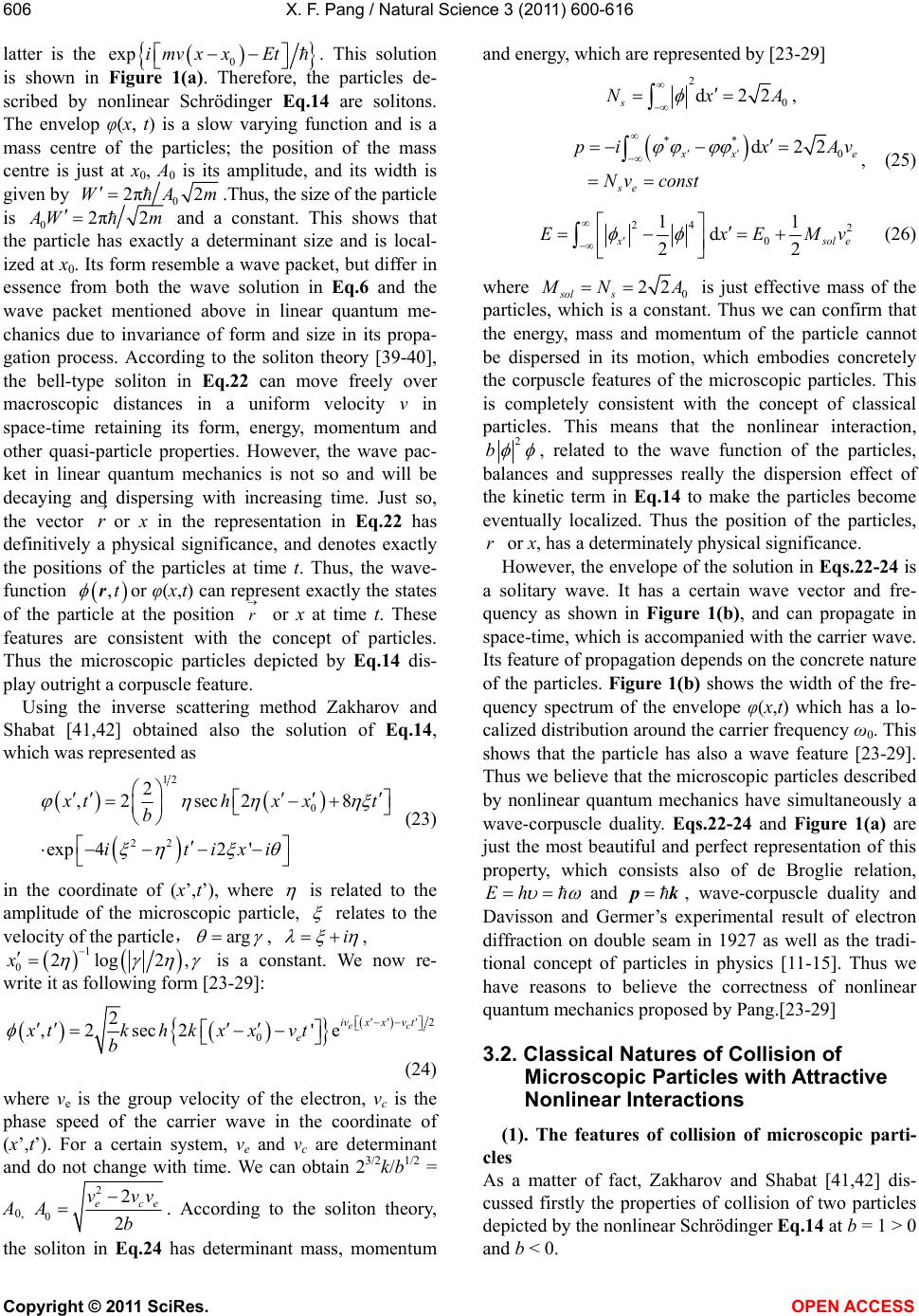

X. F. Pang / Natural Science 3 (2011) 600-616 606
latter is the


0
exp imvx xEt  

. This solution
is shown in Figure 1(a). Therefore, the particles de-
scribed by nonlinear Schrödinger Eq.14 are solitons.
The envelop φ(x, t) is a slow varying function and is a
mass centre of the particles; the position of the mass
centre is just at x
0, A0 is its amplitude, and its width is
given by 0 2π2WAm
.Thus, the size of the particle
is 02π2
A
Wm
 and a constant. This shows that
the particle has exactly a determinant size and is local-
ized at x0. Its form resemble a wave packet, but differ in
essence from both the wave solution in Eq.6 and the
wave packet mentioned above in linear quantum me-
chanics due to invariance of form and size in its propa-
gation process. According to the soliton theory [39-40],
the bell-type soliton in Eq.22 can move freely over
macroscopic distances in a uniform velocity v in
space-time retaining its form, energy, momentum and
other quasi-particle properties. However, the wave pac-
ket in linear quantum mechanics is not so and will be
decaying and dispersing with increasing time. Just so,
the vector r
or x in the representation in Eq. 22 has
definitively a physical significance, and denotes exactly
the positions of the particles at time t. Thus, the wave-
function


,t  ror φ(x,t) can represent exactly the states
of the particle at the position r



 or x at time t. These
features are consistent with the concept of particles.
Thus the microscopic particles depicted by Eq.14 dis-
play outright a corpuscle feature.
Using the inverse scattering method Zakharov and
Shabat [41,42] obtained also the solution of Eq.14,
which was represented as



12
0
22
2
,2 sec28
exp 42'
x
thxxt
b
itixi

 
 

 

 





  

(23)
in the coordinate of (x’,t’), where

is related to the
amplitude of the microscopic particle,

relates to the
velocity of the particle，arg

 , i

  ,
 
1
02log 2,x



 is a constant. We now re-
write it as following form [23-29]:
 

 2
0
2
,2sec2 'e
ec
ivxxv t
e
xtkh k xxvt
b

 
 

 
 

(24)
where v
e is the group velocity of the electron, vc is the
phase speed of the carrier wave in the coordinate of
(x’,t’). For a certain system, ve and vc are determinant
and do not change with time. We can obtain 23/2k/b1/2 =
A0,
2
0
2
2
ece
vvv
Ab

. According to the soliton theory,
the soliton in Eq.24 has determinant mass, momentum
and energy, which are represented by [23-29]
2
0
d22
s
NxA 

 

,


**
0
d22
x
xe
se
pix Av
Nv const
 


 


, (25)
24 2
0
11
d
22
x
sol e
ExEMv 





 


 (26)
where 0
22
sol s
M
NA is just effective mass of the
particles, which is a constant. Thus we can confirm that
the energy, mass and momentum of the particle cannot
be dispersed in its motion, which embodies concretely
the corpuscle features of the microscopic particles. This
is completely consistent with the concept of classical
particles. This means that the nonlinear interaction,
2
b

 , related to the wave function of the particles,
balances and suppresses really the dispersion effect of
the kinetic term in Eq.14 to make the particles become
eventually localized. Thus the position of the particles,
r or x, has a determinately physical significance.
However, the envelope of the solution in Eqs.22-24 is
a solitary wave. It has a certain wave vector and fre-
quency as shown in Figure 1(b), and can propagate in
space-time, which is accompanied with the carrier wave.
Its feature of propagation depends on the concrete nature
of the particles. Figure 1(b) shows the width of the fre-
quency spectrum of the envelope φ(x,t) which has a lo-
calized distribution around the carrier frequency ω0. This
shows that the particle has also a wave feature [23-29].
Thus we believe that the microscopic particles described
by nonlinear quantum mechanics have simultaneously a
wave-corpuscle duality. Eqs.22-2 4 and Figure 1(a) are
just the most beautiful and perfect representation of this
property, which consists also of de Broglie relation,
Eh


 and

pk, wave-corpuscle duality and
Davisson and Germer’s experimental result of electron
diffraction on double seam in 1927 as well as the tradi-
tional concept of particles in physics [11-15]. Thus we
have reasons to believe the correctness of nonlinear
quantum mechanics proposed by Pang.[23-29]
3.2. Classical Natures of Collision of
Microscopic Particles with Attractive
Nonlinear Interactions
(1). The features of collision of microscopic parti-
cles
As a matter of fact, Zakharov and Shabat [41,42] dis-
cussed firstly the properties of collision of two particles
depicted by the nonlinear Schrödinger Eq.14 at b = 1 > 0
and b < 0.

X. F. Pang / Natural Science 3 (2011) 600-616 607
Figure 1. The solution of Eq.14 and its features.
According to Lax method [43], if two linear operators

L and

B corresponding to Eq.14,which depend on

, satisfy the following Lax operator equation:
ˆˆˆˆˆ ˆ
,
t
iLBLLBB L



where

B is a self-adjoint operator, then the eigenvalue
k and eigenfunction  of the operator

L satisfy the
equation:
ˆ
Lk   with

1
2
,xt 






, (27)
but

B satisfies the equation: ˆt Bi

 .
Zakharov and Shabat [41,42] found out that the con-
crete representations of

L and

B for Eq.14, which
are as follows
2
2
22
10 0
ˆ01 0
10 1
ˆ01
1
x
x
s
Li sx
i
s
Bs x
i
s









 









 

 
 
 
 




, (28)
where

212
s
b ，

,t  rsatisfies Eq.14. We rep-
resent  in Eq.28 in one-dimensional case by

expSikx


  (29)
where


12
12
01
10
s
S
s






，22
1
k
kbk
s

.
Inserting Eq.91 and

L in Eq.90 into Eq .2 7 the
Zakharov-Shabat (ZS) equation [41,42] can be obtained
as follows:
12 1xqi


 (30)
212xqi



 (31)
where

1
2
12
22
1
ib
qi
s






, ks
 .
Zakharov and Shabat found out the soliton solution of
Eq.14 using the inverse scattering method from ZS Eqs.
30 and 31, which is denoted in Eq.22, and studied fur-
ther the properties of collision of these soliton solutions
in these cases. In the studies of b = 1 > 0, they gave first
this single soliton solution of this equation, where
22

is the amplitude of the soliton, 22

denotes
its velocity, i



 is the eigenvalues of the
linear operator

L in Eq.90, 0
x
 and

 are the mass
centre and phase of microscopic particle. In such a case
they found further out the N-soliton solution of Eq.15
and studied thus the collision features of two solitons in
the system. We here adopted their results of research to
explain the rules and properties of collision between the
microscopic particles in the nonlinear quantum mechan-
ics. They [41,42] find from calculation that the mass
centre and phase of particle occur only change after this
collision. The translations of the mass centre 0m
x


and
phase m


of mth particles, which moves to a positive
direction after this collision, can be represented, respec-
tively, by
00 *
1
*
1
10, and
2arg
Nmp
mm
pm
mmp
Nmp
mm
pm mp
xx



 






 



 





(32)
where m

and m

are some constants related to the
amplitude and eigenvalue of mth particles, respectively.
The equations show that shift of position of mass centre
of the particles and their variation of phase are a con-
stants after the collision of two particles moving with
different velocities and amplitudes. The collision process
of the two particles can be described from Eq.32 as fol-
lows. Before the collision and in the case of t


the slowest soliton is in the front while the fastest at the
rear, they collide with each other at t’=0, after the colli-
sion and t

, they are separated and the positions
just reversed. Thus Zakharov and Shabat[ 41-42] obtained
that as the time t varies from  to , the relative
change of mass centre of two particles, 0m
x
 , and their
relative change of phases, m

, can, respectively, de-

X. F. Pang / Natural Science 3 (2011) 600-616 608
noted as
000
1
**
11
1ln ln
mmm
Nm
mpmp
km k
mmpmp
xxx







 

 


 




(33)
and
1
**
11
2arg2arg
mmm
mN
mp mp
kkm
mp mp

















(34)
where 0m
x

 and phase m

 are the mass centre and
phase of mth particles at inverse direction or initial posi-
tion, respectively. Eq.34 can be interpreted by assuming
that the microscopic particles collide pair wise and every
microscopic particle collides with others. In each paired
collision, the faster microscopic particle moves forward
by an amount of

1*
ln
mmkmk

 
, mk

 , and the slower one
shifts backwards by an amount of

1*
ln
kmkmk

 
. The total shift is equal to the
algebraic sum of their shifts during the paired collisions.
So that there is no effect of multi-particle collisions at all.
In other word, in the collision process in each time the
faster particle moves forward by an amount of phase
shift, and the slower one shifts backwards by an amount
of phase. The total shift of the particles is equal to the
algebraic sum of those of the pair during the paired col-
lisions. The situation is the same with the phases. This
rule of collision of the microscopic particles described
by the nonlinear Schrödinger Eq.14 is the same as that
of classical particles, or speaking, meet also the collision
law of macroscopic particles, i.e., during the collision
these microscopic particles interact and exchange their
positions in the space-time trajectory as if they had
passed through each other. After the collision, the two
microscopic particles may appear to be instantly trans-
lated in space and/or time but otherwise unaffected by
their interaction. The translation is called a phase shift as
mentioned above. In one dimension, this process results
from two microscopic particles colliding head-on from
opposite directions, or in one direction between two par-
ticles with different amplitudes or velocities. This is
possible because the velocity of a particle depends on
the amplitude. The two microscopic particles surviving a
collision completely unscathed demonstrate clearly the
corpuscle feature of the microscopic particles. This
property separates the microscopic particles (solitons)
described by the nonlinear quantum mechanics from the
particles in the linear quantum mechanical regime. Thus
this demonstrates the classical feature of the microscopic
particles.
(2). The results of numerical simulation of collision
of microscopic particles
Pang et al..[23- 29,44] who further simulated numeri-
cally the collision behaviors of two particles described
nonlinear Schrödinger Eq.8 at V(x) = constant and


0A 

using the fourth-order Runge_Kutta me-
thod[45-46].
For the purpose we now divide Eq.8 at


0A 

and b > 0 in one-dimensional case into the following
two-equations
22
2,
2
u
itm x
x









 (35)

22 2
0
22 .
uu
Mv x
tx







 (36)
Eqs.35 and 36 describe the features of motion of
studied soliton and another particle ( such as, phonon) or
background field (such as, lattice) with mass M and ve-
locity v0, respectively, where u is the characteristic quan-
tity of another particle (as phonon) or of vibration (such
as, displacement) of the background field. The coupling
between the two modes of motion is caused by the de-
formation of the background field through the studied
soliton – background field coupling, such as, di-
pole-dipole interaction,

is the coupling coefficient
between them and represents the change of interaction
energy between the studied soliton and background field
due to an unit variation of the background field. The
relation between the two modes of motion can be ob-
tained from Eq.36 and represented by

2
22
0
u
A
xMv v
 


 (37)
If inserting Eq.37 into Eq.35 yields just the nonlinear
Schrödinger Eq.8 at V(x) = constant, where

2
22
0
b
M
vv

 is a nonlinear coupling coefficient,


VxA

, A is an integral constant. This result shows
clearly that the nonlinear interaction
2
b

 comes
from the coupling interaction between the studied soliton
and background field. This is the reason what 2 b

 is
referred to as nonlinear interaction.
In order to use fourth–order Runge-Kutta method[45-46].
to solve numerically Eqs.35 and 36 we must further dis-
cretize them, thus they are now denoted as
  
  
.
11
01 1
2
nnnn
nnn
ittJ tt
ru tu tt
 



  



 (38)
 

..
11
22
01 1
2
2
nnnn
nn
M
utWutut ut
r 










(39)

X. F. Pang / Natural Science 3 (2011) 600-616 609
where
 
n
n
t
tt




,
 
2
..
2
n
n
ut
ut t

 and the follow-
ing transformation relation between continuous and dis-
crete functions are used
 
,n
x
tt   and
 
,n uxtu t,
  
2
2
100
2
1
2!
nn
nn
tt
ttr r
xx




 

  
2
2
100
2
1
2!
nn
nn
ut ut
ututr r
xx


 
 (40)
where 22222
0000
,2,mrAJmrWM vr    ,
0
r is distance between neighboring two lattice points. If
using transformation:


exp
nn it
   we can
eliminate the term


nt
 in Eq.38. Again making a
transformation:








nnn n
tatatriati   , then
Eqs.38 and 39 become
 
11 011
2
nnn nnn
arJaiairuuai 
 
 

 (41)

11 011
2
nnn nnn
aiJararruuar 
 
 

 (42)
.
nn
uyM (43)




11
22 22
01111
2
2
nnnn
nnnn
yWuuu
raraiar ai 





(44)
2222
nnnn
aarai


(45)
where arn and ain are real and imaginary parts of an.
Eqs.41-45 can determine states and behaviors of the
microscopic particle. Their solutions can be found out
from the four equations. There are four equations for one
structure unit. Therefore, for the quantum systems con-
structed by N structure units there are 4N associated
equations. When the fourth-order Runge-Kutta method
[45,46] is used to numerically calculate these solutions
we must further discretize them, in which n is replaced
by j and let the time be denoted by n, the step length of
the space variable is denoted by h in the above equations.
An initial excitation is required in this calculation, which
is chosen as, an(o)=ASech[(n-n0)

2
0
24JWr  ]
(where A is the normalization constant) at the size n, for
the applied lattice, un(0) = yn(0) = 0. In the numerical
simulation it is required that the total energy and the
norm (or particle number) of the system must be con-
served. The system of units, ev for energy, 0
A for
length and ps for time are proven to be suitable for the
numerical solutions of Eqs.41-44. The one dimensional
system is composed of N units and fixed, where N is
chosen to be N = 200, and a time step size of 0.0195 is
used in the simulations. Total numerical simulation is
performed through data parallel algorithms and MALAB
language.
If the values of the parameters, ,,, ,MJW

 and
0
r in Eqs.38 and 39 are appropriately chosen we can
calculate the numerical solution of the associated
Eqs.41-44 by using the fourth-order Runge-Kutta
method [45,46], thus the changes of
 
22
nn
tat  ,
which is probability or number density of the particle
occurring at the nth structure unit, with increasing time
and position in time-place can be obtained. This result is
shown in Figure 3, which shows that the amplitude of
the solution can retain constancy in motion process, i.e.,
the solution of Eqs.38 and 39 or Eq.8 at V(x) = constant
is very stable while in motion. In the meanwhile, we
give the propagation feature of the solutions of Eqs.41-
44 in the cases of a long time period of 250ps and long
spacings of 400 in Figure 3, which indicates that the
states of solution are also stable in the long propagation.
According to the soliton theory [39,40] we can obtain
that Eqs.38 and 39 have exactly a soliton solution,
which have a feature of classical particles.
In order to verify the corpuscle feature of the solution
of nonlinear Schrödinger Eq.8 we study their collision
property in accordance with the soliton theory[39-40]. Thus
we further simulated numerically the collision behaviors
of two solitonn solutions of Eq.8 at
V(x) =2
0
mr A

  = constant using the fourth-order
Runge-Kutta method[45-46]. This process resulting from
two particles colliding head-on from opposite directions,
which are set up from opposite ends of the channel, is
shown Figure 4, where the above initial conditions si-
multaneously motivate the opposite ends of the channels.
From this figure we see clearly that the initial two parti-
cles having clock shapes and separating 50 unit spacings
in the channel collide with each other at about 8 ps and
25 units. After this collision, the two solitons in the
channel go through each other without scattering ob-
tained by Zakharov and Shabat [41,42] as mentioned
above. Clearly, the property of collision of the and retain
their clock shapes to propagate toward and separately
along itself channels. The collision properties of the
solitons described by the nonlinear Schrödinger Eq.8 are
same with those solutions of Eq.8 is same with the rules
of collision of macroscopic particles. Thus, we can con-
clude that microscopic particles described by nonlinear
Schrödinger Eq . 8 have a corpuscle feature.
However, we see clearly that there is a wave peak with
large amplitude in the colliding process in Figure 4.
Obviously, this is a result of complicated superposition of
solitary waves of two particles. This result displays the
wave feature of the particles. Therefore, the collision
process shown in Figure 3 represent obviously that the
soliton solutions of the nonlinear Schrödinger equation
have a both corpuscle and wave feature, which is due to
the nonlinear interaction 2 b

 .

X. F. Pang / Natural Science 3 (2011) 600-616 610
One words, the above properties of propagation and
collision of particles described by the nonlinear
Schrödinger equation with an external applied potential
show that the particles are stable in propagation, and they
can go through each other retaining their form after the
collision of head-on from opposite directions, This fea-
ture is the same with that of the classical particles.
However, a wave peak with large amplitude, which is a
result of complicated superposition of two solitary waves,
occur in the colliding process. This displays the wave
feature of the solitons. Therefore, the collision property
of the solitons shows clearly that the solutions of the
nonlinear Schrödinger equation have a both corpuscle
and wave feature. Obviously, this is due to the nonlinear
Figure 2. Motion of soliton solution of Eqs.38 and 39.
Figure 3. State of motion of microscopic particle described by Eqs.38 and 39 in the cases of a long time period
and long spacings.
Figure 4. the features of collision of microscopic particles.

X. F. Pang / Natural Science 3 (2011) 600-616 611
interaction 2
b


,, which suppresses the dispersive
effect of kinetic energy in the dynamic equation. Thus the
microscopic particles have a wave-corpuscle duality in
this case.
3.3. The Uncertainty Relationship for the
Position and Momentum
(1). Correct form of uncertainty relation in the
linear quantum mechanics
As it is known, the microscopic particle has not a de-
terminant position, disperses always in total space in a
wave form in the linear quantum mechanics. Hence, the
position and momentum of the microscopic particles
cannot be simultaneously determined. This is just the
well-known uncertainty relation. The uncertainty rela-
tion is an important formulae and also an important
problem in the linear quantum mechanics that troubled
many scientists. Whether this is an intrinsic property of
microscopic particle or an artifact of the linear quantum
mechanics or measuring instruments has been a long-
lasting controversy. Obviously, it is closely related to
elementary features of microscopic particles. Since we
have established the nonlinear quantum mechanics, in
which the natures of the microscopic particles occur
considerable variations relative to that in the linear quan-
tum mechanics, thus we expect that the uncertainty rela-
tion in nonlinear quantum mechanics could be changed
relative to that in the linear quantum mechanics. Then
the significance and essence of the uncertainty relation
can be revealed by comparing the results of linear and
nonlinear quantum theories.
The uncertainty relation in the linear quantum me-
chanics can be obtained from [25-29,47]



2
ˆˆ
I'A+iB,td0  
 
rr
or
 
*ˆ
ˆˆ
F=,t FA,t ,B,t,t d  


rrrrr
 (46)
In the coordinate representation,


and
A
B are op-
erators of two physical quantities, for example, position
and momentum, or energy and time, and satisfy the
commutation relation ˆˆ
ˆ
,
A
BiC


 ,

,t  r and

,t 
rare wave functions of the microscopic particle
satisfying the Schrödinger equation 1.7 and its conju-
gate equation, respectively,
 

2
ˆ
F=A'+ B,  
(ˆˆˆˆ A=AA, B=BB, A and B are the average values
of the physical quantities in the state denoted by

,t  r), is an operator of physical quantity related to
A and B ,

is a real parameter. After some simplifica-
tions, we can get from Eq.46
22 2
22 2
ˆˆ
ˆˆ
I=F=A2ABB0or
ˆˆˆ
A'C'B0


 

(47)
Using mathematical identities, this can be written as
22 2
ˆˆ ˆ
AB C4
 (48)
This is the uncertainty relation which is often used in
the linear quantum mechanics. From the above deriva-
tion we see that the uncertainty relation was obtained
based on the fundamental hypotheses of the linear quan-
tum mechanics, including properties of operators of the
mechanical quantities, the state of particle represented
by the wave function, which satisfies the Schrodinger

Eq.2, the concept of average values of mechanical quan-
tities and the commutation relations and eigenequation
of operators. Therefore, we can conclude that the uncer-
tainty relation in Eq.48 is a necessary result of the
quantum mechanics. Since the linear quantum mechan-
ics only describes the wave nature of microscopic parti-
cles, the uncertainty relation is a result of the wave fea-
ture of microscopic particles, and it inherits the wave
nature of microscopic particles. This is why its coordi-
nate and momentum cannot be determined simultane-
ously. This is an essential interpretation for the uncer-
tainty relation Eq.48 in the linear quantum mechanics. It
is not related to measurement, but closely related to the
linear quantum mechanics. In other words, if the linear
quantum mechanics could correctly describe the states of
microscopic particles, then the uncertainty relation
should also reflect the peculiarities of microscopic parti-
cles.
Eq.48 can be written in the following form [25-29,47]:



2
22
2
22
ˆˆˆ ˆˆ
F=A'AB /A
ˆˆ ˆˆ
BABA0
 

 
(49)
or


22
2222
ˆˆ ˆˆˆ ˆ
A4AB4A0CC 


  (50)
This shows that 2
ˆ
A0

, if

2
ˆˆ
AB  or 2
ˆ4C is
not zero, else, we cannot obtain Eq.48 and


2
22
ˆˆ
ABAB  because when 2
ˆ0
A , Eq.50
does not hold. Therefore,

2
ˆ0A
 is a necessary
condition for the uncertainty relation Eq.48, 2
ˆ
A

can
approach zero, but cannot be equal to zero. Therefore, in
the linear quantum mechanics, the right uncertainty rela-
tion should take the form:

2
22 2
ˆˆ
ˆ4AB C  (51)

X. F. Pang / Natural Science 3 (2011) 600-616 612
(2). Uncertainty relation of microscopic particle in
nonlinear quantum mechanics
We now return to study the uncertainty relation of the
microscopic particles described by the nonlinear quan-
tum mechanics. In such a case the microscopic particles
is a soliton and have a wave-corpuscle duality. Thus we
have the reasons to believe that the uncertainty relation
in this case should be different from equation (115) in
the linear quantum theory.
Pang [26-29,67] derived this relation for position and
momentum of a microscopic particle depicted by the
nonlinear Schrödinger Eq.14 with a solution,
s

, as
given in Eq.22. The function

,
s
x
t 
 is a square in-
tegral function localized at 00x in the coordinate
space. The Fourier transform of this function is given by
 
1
,,ed
2π
ip x
ss
ptxtx 



 
 (52)
Using Eq.22 , then the Fourier transform is explicitly
represented as


 

22 '
0
ππ
,sech 22
242
exp42 2)' 2 2
spt p
iptipxi



 

 



 
(53)
It shows that

,
spt

 is also localized at p in mo-
mentum space. Eqs.22 and 53 show that the microscopic
particle is localized in the shape of soliton not only in
position space but also in the momentum space. For
convenience, we introduce the normalization coefficient
0
B
in Eqs.22 and 53, then obviously 242
o
B  , the
position of the mass center of the microscopic particle,
x
, and its square,
2, 0xatt

are given by
 
22
22
d, d
ss
x
xxxxx xx 

 



. (54)
We can thus find that
22
22 22
0
000 0
π
42, 42
12 2
A
x
AxxA x




 (55)
respectively. Similarly, the momentum of the mass cen-
ter of the microscopic particle, p, and its square ,
2
p, are given by
 
22
22
ˆˆ
d, d
ss
pp pppppp 

 
 


(56)
which yield
2223 23
000
322
16, + 322
3
pA pAA



 (57)
The standard deviations of position
2
2 xxx

 and momentum
2
2
ppp


 are given by




22
2222
00 0
2
223322
00
ππ
4142 ,
12 96
18
32 214 2,
33
xA xA
pAA



 







 


(58)
respectively. Thus Pang [27-29,47] obtain the uncer-
tainty relation between position and momentum for the
microscopic particle depicted by the nonlinear
Schrödinger equation in Eq.15
π6xp



 (59)
This result is not related to the features of the micro-
scopic particle (soliton) depicted by the nonlinear
Schrödinger equation because Eq.59 has nothing to do
with characteristic parameters of the nonlinear
Schrödinger equation. π in Eq. 59 comes from of the
integral coefficient 12π. For a quantized micro-
scopic particle, π in Eq.59 should be replaced by
π,because Eq.52 is replaced by
 
1
,d,e.
2π
ipx
ss
ptx xt 



 (60)
Thus the corresponding uncertainty relation of quan-
tum microscopic particle is given by[24-27,47]
π612xp h

  (61)
This uncertainty principle also suggests that the posi-
tion and momentum of the microscopic particle can be
simultaneously determined in a certain degree. It is pos-
sible to estimate roughly the sizes of the uncertainty of
these physical quantities. If it is required that


s,tx


in Eq.22 or


s
p
,t 
in Eq.53 satisfies the
admissibility condition i.e.,

s00
 ,we choose
140, =3000.25322   and 00
x in Eq .22
(In fact, in such a case we can get

7
s010


, thus the
admissibility condition can be satisfied). We then get
0.02624 x


 and 19.893,p


according to Eqs.59
and 60. This result shows that the position and momen-
tum of the microscopic particles in the nonlinear quan-
tum mechanics could be determined simultaneously
within a certain approximation, one of these cannot ap-
proach infinite.
Also, the uncertainty relation in Eq.61 or Eq.59 differ
from the 2xp

 in Eq.61 in the linear quantum
mechanics. However, the minimum value 2xp 
has not been obtained from both the solutions of linear
Schrödinger equation and experimental measurement up
to now, except for the coherent and squeezed states of

X. F. Pang / Natural Science 3 (2011) 600-616 613
microscopic particles. Therefore we can draw a conclu-
sion that the minimum uncertainty relationship is a
nonlinear effect, instead of linear effect, and a result of
wave-corpuscle duality.
From this result we see that when the microscopic
particles satisfy 2xp , then their motions obey
laws of the linear quantum mechanics, the particles are
some waves. When the uncertainty relationship of
12 or π6 xp  is satisfied, the microscopic par-
ticles should be described by nonlinear quantum me-
chanics, and have a wave-corpuscle duality. If the posi-
tion and momentum of the particles meets 0xp ,
then the particles have only a corpuscle feature, i.e., they
are the classical particles. Therefore, the minimum un-
certainty relation in Eqs.61 and 59 exhibits clearly the
wave-corpuscle duality of microscopic particles de-
scribed by nonlinear quantum mechanics, which bridges
also the gap between the classical and linear quantum
mechanics. This is a very interesting result in physics.
(3). The uncertainty relations of the coherent states
As a matter of fact, we can represent one-quantum
coherent state of harmonic oscillator by[48]

22
0
ˆˆˆ
exp0 e0
1
n
n
n
bb b
n




 


,
in the number picture, which is a coherent superposition
of a large number of quanta. Thus
 
ˆˆ
,
2
xpim
m




 
,
and


222
222
ˆ21,
2
ˆ21
2
xm
m
p
 


 





,
where
 
ˆˆˆˆ
ˆ ˆ, p=i,
22
m
x
bbbb
m





and

ˆˆ
bb
 is the creation (annihilation) operator of
microscopic particle (quantum),

and

 are some
unknown functions,

is the frequency of the particle,
m is its mass. Thus we can get
 
2
2222
m
,p,x p
22 4
xm


 
 
(62)
This is a minimum uncertainty relationship for the
coherent state.
For the squeezed state of the microscopic particle:

+2 2
expbb0 



, which is a two quanta cohe-
rent state, we can find that
242 4
m
e, pe
2m 2
x



 


 

,
using a similar approach as the above. Here

is the
squeezed coefficient and 1  . Thus,
8
1
, e,
2
x
xp pm



 

 or

8
epxm



 (63)
This shows that the squeezed state meets a minimum
uncertainty relationship, the momentum of the micro-
scopic particle (quantum) is squeezed in the two-quanta
coherent state compared to that in the one-quantum co-
herent state.
The above results show that both one-quantum and
two-quanta coherent states satisfy the minimal uncer-
tainty principle. This is the same with that of the micro-
scopic particles in the nonlinear quantum mechanics.
This means that coherent and squeezed states are a
nonlinear quantum state, the coherence and squeezing of
quanta are a kind of nonlinear quantum effect. Just so,
the states of a microscopic particles described by the
nonlinear Schrödinger Eq.8 , such as the Davydov’s
wave functions [49], both 12
ID> and ID>, and Pang’s
wave function of exciton-solitons[50-53] in protein mole-
cules and acetanilide; the wave function of proton trans-
fer in hydrogen-bonded systems and the BCS’s wave
function in superconductors [34], etc., are always repre-
sented by a coherent state. Hence, the coherence of par-
ticles does not belong to the systems described by linear
quantum mechanics, because the coherent state cannot
be obtained by superposition of linear waves, such as
plane wave, de Broglie wave, or Bloch wave. Then the
minimal uncertainty relation Eq.61 , as well as Eqs.59
and 63, are only applicable to microscopic particles de-
scribed by the nonlinear quantum mechanics. Thus it
reflects the wave-corpuscle duality of the microscopic
particles.
Also, the above results indicate not only the essences
of nonlinear quantum effects of the coherent state or
squeezing state but also that the minimal uncertainty
relationship is an intrinsic feature of the nonlinear quan-
tum mechanics systems including the coherent and
squeezing states.
Pang et al. [50-53] also calculated the uncertainty re-
lationship and quantum fluctuations and studied their
properties in nonlinear electron-phonon systems based
on the Holstein model by a new ansatz including the
correlations among one-phonon coherent and two-pho-
non squeezing states and polaron state. Many interesting
results were obtained, such as the minimum uncertainty
relationship is related to the properties of the micro-
scopic particles. The results enhanced the understanding
of the significance and essences of the minimum uncer-
tainty relationship.

X. F. Pang / Natural Science 3 (2011) 600-616 614
4. CONCLUSIONS, RESOLUTION OF
DIFFICULTIES OF LINEAR QUANTUM
MECHANICS
As it is known, the states and properties of micro-
scopic particle were described by the linear Schrödinger
Eq.3 in the quantum mechanics, but the microscopic
particles have only a wave feature, not corpuscle feature
as described in Introduction. In nonlinear quantum me-
chanics, we have broken through the hypothesis of in-
dependence of Hamiltonian operator of the systems on
states of microscopic particles, forsaken the above line-
arity hypothesis of linear quantum mechanics and taken
into account the true motions of each particle and back-
ground field and the interactions between them, thus the
microscopic particles accepted a nonlinear interaction
and their laws of motion are then described by Eqs.8-13
Thus natures and properties of the microscopic particles
appear considerable changes, when compared with those
in linear quantum mechanics. The changes can be sum-
marized as follows [17-37].
1) In this new theory although the states of micro-
scopic particles are still represented as a wave function

t  r, in Eq.7, its absolute square,
 
22
ttt  r,r,r, , denotes no longer the pro-
bability of finding the microscopic particle at a given
point in the space-time, and give just the mass density of
the microscopic particles at that point. Thus we can find
out the particle number or the mass of the particle from
2dN


 
, the concept of probability is abandoned
thoroughly in nonlinear quantum mechanics. Then the
difficulty of statistical interpretation for the wave func-
tion of microscopic particle in quantum mechanics is
solved .
2) The dynamic equations the particles satisfy are not
the linear Schrödinger equation in Eq.2 and linear
Klein-Gordon equation, but nonlinear Schrödinger equa-
tions in Eqs. 8 and 9 and nonlinear Klein-Gordon equa-
tions in Eqs.10 and 11. Their solutions have a wave-
corpuscle duality, which is embedded by organic com-
bination of envelope and carrier wave as shown in Fig-
ure 1. In such a case the particle has not only a wave
feature, such as a certain amplitude, velocity, frequency,
and wavevector, but also corpuscle natures, such as, a
determinant mass centre, size, mass, momentum and
energy. This is the first time to explain physically the
wave- corpuscle duality of microscopic particles in
quantum systems. This is a great advance of modern
quantum theory, thus it solved a most great difficulty of
one century existed in quantum mechanics.
3) In nonlinear quantum mechanics, *dx




,
*dx
t





 and

*d
H
x


 or

H

 are no
longer some average values of the physical quantities in
linear quantum mechanics, but represent the position,
velocity and acceleration of the mass center and energy
of the microscopic particles, respectively, and have de-
terminant values. Thus, the presentations of physical
quantities in the nonlinear quantum mechanics appear
considerably the variations relative to those in linear
quantum mechanics. This has solved the difficulty aris-
ing from the average values, which represent the physi-
cal quantities in linear quantum mechanics.
4) The microscopic particles have determinant mass,
momentum and energy, and obey universal conservation
laws of mass, momentum, energy and angular momen-
tum. This amount to bridge over the gap between the
classical mechanics and linear quantum mechanics.
5)The microscopic particles meet the classical colli-
sion rule, when they collide with each other. Although
these particles are deformed in the collision, which de-
notes its wave feature, they can still retain their form and
amplitude to move towards after collision, where a phase
shift occurs only. This denotes that the microscopic par-
ticles in nonlinear quantum mechanics possess both
corpuscle and wave property, but the corpuscle property
differs from classical particles.
6) The position and momentum of the mass centre of
microscopic particles are determinant, but their uncer-
tainties obey only to a minimal uncertainty relation due
to the wave-corpuscle duality, which differs from those
in linear quantum mechanics. This means that the coor-
dinate and momentum of microscopic particles may be
simultaneously determined at a certain degree. This
amount to bridge over the gap between the classical
mechanics and linear quantum mechanics.
These show clearly the necessity, validity and impor-
tance of establishing nonlinear quantum mechanics.
Thus the difficulties of linear quantum mechanics can be
also solved thoroughly by nonlinear quantum mechanics.
Therefore, to develop and to establish NLQM can solve
problems disputed by scientists in the LQM field for
about a century [7-9], can promote the development of
physics and enhance and raise the knowledge and recog-
nition levels to the essences of microscopic matter. We
can predict that nonlinear quantum mechanics has exten-
sive applications in physics, chemistry, biology, poly-
mers, etc.
5. ACKNOWLEDGEMENTS
I would like to acknowledge the Major State Basic Research Devel-
opment Program (973 program) of China for the financial support

X. F. Pang / Natural Science 3 (2011) 600-616 615
(grate No: 212011CB503 701).
REFERENCES
[1] Bohr, D. and Bub, J. (1966) A proposed solution of the
measurement problem in quantum mechanics. Review of
morden Physics, 6, 453-469.
doi:10.1103/RevModPhys.38.453
[2] Schrödinger, E. (1935) Die gegenwartige situation in der
quantenmechanik, Naturwissenschaften, 23, 807-849.
doi:10.1007/BF01491891
[3] Schrödinger, E. (1935) The present situation in quantum
mechanics, a translation of translation of Schrodinger.
Proceedings of the American Philosophical Society, 124,
323-338.
[4] Schrödinger, E. (1926) An undulatory theory of the me-
chanics of atoms and molecules. Physical Review, 28,
1049-1070. doi:10.1103/PhysRev.28.1049
[5] Heisenberg, W. Z. (1925) Über die quantentheoretische
umdeu- tung kinematischer und mechanischer beziehun-
gen. Zeitschrift der Physik, 33, 879-893.
doi:10.1007/BF01328377
[6] Heisenberg, W. and Euler, H. (1936) Folgerungen aus der
Diracschen Theorie des Positrons. Physics and Astronomy,
98, 714-732. doi:10.1007/BF01343663
[7] Born, M. and Infeld, L. (1934) Foundations of the New
Field Theory, Proceedings of the American Philosophical
Society, 144, 425.
[8] Dirac, P.A.M. (1948) Quantum Theory of Localizable
Dynamical Systems, Physical Review, 73, 1092.
doi:10.1103/PhysRev.73.1092
[9] Diner, S., Farque, D., Lochak, G., and Selleri, F. (1984)
The wave-particle dualism. Riedel, Dordrecht.
[10] Ferrero, M. and Van der Merwe, A. (1997) New devel-
opments on fundamental problems in quantum physics.
Kluwer, Dordrecht.
[11] Ferrero, M. and Van der Merwe, A. (1995) Fundamental
problems in quantum physics. Kluwer, Dordrecht.
[12] de Broglie, L., (1960) Nonlinear wave mechanics: A
causal interpretation, Elsevier, Amsterdam.
[13] de Broglie, L., (1955) Une interpretation nouvelle de la
mechanique ondulatoire: Est-elle possible? Nuovo Cimento,
1, 37-50.
[14] Bohm, D.A. (1952) Suggested interpretation of the
quantum theory in terms of ‘hidden’ variables. Physical
Review, 85, 166-180.
[15] Potter, J. (1973) Quantum mechanics. North-Holland
publishing Co. Amsterdam.
[16] Jammer, M. (1989) The concettual development of
quantum mechanics. Tomash Publishers, Los Angeles.
[17] Einstein, A., Podolsky, B. and Rosen, N. (1935) The
appearance of this work motivated the present–shall I say
lecture or general confession? Physical. Review, 47,
777-780. doi:10.1103/PhysRev.47.777
[18] Einstein, A.P., (1979) A centenary Volume. Harvard Uni-
versity Press, Cambridge.
[19] Pang, X.F. (1985) Problems of nonlinear quantum me-
chanics. Sichuan Normal University Press, Chengdu.
[20] Pang, X.F. (2008) The Schrodinger equation only descry-
bes approximately the properties of motion of micro-
scopic particles in quantum mechanics. Nature Sciences,
3, 29.
[21] Pang, X.F. (1985) The fundamental principles and theory
of nonlinear quantum mechanics. China Journal of Po-
tential Science, 5, 16.
[22] Pang, X.F. (1982) Macroscopic quantum mechanics.
China Nature Journal, 4, 254.
[23] Pang, X.F. (1986) Bose-condensed properties in super-
con-ducors. Journal of Science Exploration, 4, 70.
[24] Pang, X.F. (1991) The theory of nonlinear quantum me-
chanics: In research of new sciences, Science and
Techbology Press, Hunan, 16-20.
[25] Pang, X.F. (2008) The wave-corpuscle duality of micro-
scopic particles depicted by nonlinear Schrodinger equa-
tion. Physica B, 403, 4292-4300.
doi:10.1016/j.physb.2008.09.031
[26] Pang, X.F. (2008) Features and states of microscopic
particles in nonlinear quantum–mechanics systems. Fron-
tiers of physics in China, 3, 413.
[27] Pang, X.F. (2005) Quantum mechanics in nonlinear sys-
tems. World Scientific Publishing Co., Singapore.
doi:10.1142/9789812567789
[28] Pang, X.F. (2009) Nonlinear quantum mechanics. China
Electronic Industry Press, Beijing.
[29] Pang, X.F. (1994) The Theory of nonlinear quantum
mechanics. Chinese Chongqing Press, Chongqing.
[30] Pang, X.F. (2006) Establishment of nonlinear quantum
mechanics. Research and Development and of World
Science and Technology, 28, 11.
[31] Pang, X.F. (2003) Rules of motion of microscopic parti-
cles in nonlinear systems. Research and Development
and of World Science and Technology, 24, 54.
[32] Pang, X.F. (2006) Features of motion of microscopic
particles in nonlinear systems and nonlinear quantum
mechanics in sciencetific proceding-physics and others.
Atomic Energy Press, Beijing.
[33] Parks, R. D. (1969) Superconductivity. Marcel, Dekker.
[34] Josephson, D.A. (1965), Supercurrents through barriers,
Advanced Physics, 14, 39-451.
[35] Suint-James, D. et al., (1966) Type-II superconductivity,
Pergamon, Oxford.
[36] Bardeen, L.N., Cooper L.N. and Schrieffer, J. R. (1957)
Superconductivity theory. Physical Review, 108, 1175-
1204. doi:10.1103/PhysRev.108.1175
[37] Barenghi, C.F., Donnerlly, R.J. and Vinen, W.F. (2001)
Quantized vortex dynamics and superfluid turbulence.
Springer, Berlin. doi:10.1007/3-540-45542-6
[38] Donnely, R.J. (1991) Quantum vortices in heliem II.
Cambridge University Press, Cambridge.
[39] Pang, X.F. (2003) Soliton physics. Sichuan Science and
Technology Press, Chengdu.
[40] Guo, B.L. and Pang, X.F. (1987) Solitons. Chinese Sci-
ence Press, Beijing.
[41] Zakharov, V.E. and Shabat, A.B. (1972) Exact theory of
two-dimensional self-focusing and one-dimensional self-
domulation of wave in nonlinear media. Soviet Physics
JETP, 34, 62.
[42] Zakharov, V.E. and Shabat, A.B. (1973) Interaction be-
tween solitons in a stable medium. Soviet Physics JETP,
37, 823
[43] Lax, P.D. (1992) Integrals of nonlinear equations of evo-
lution and solitary waves, Cambridge University Press,
Cambridge, 107-351

X. F. Pang / Natural Science 3 (2011) 600-616 616
[44] Pang, X.F. (2010) Collision properties of microscopic
particles described by nonlinear Schrodinger equation.
International Journal of Nonlinear science and numeri-
cal Simulation, 11 , 1069-1075.
[45] Stiefel, J. (1965) Einfuhrung in die numerische mathe-
matik. Teubner Verlag, Stuttgart.
[46] Atkinson, K.E. (1987) An Introdution to numerical
analysis. Wiley, New York.
[47] Pang, X.F. (2009) Uncertainty features of microscopic
particles described by nonlinear SchrÖdinger equation.
Physica B, 405, 4327-4331.
doi:10.1016/j.physb.2009.08.027
[48] Glanber, R.J. (1963) Coherent and incoherent states of
the radiation field. Physical Review, 13, 2766-2788.
doi:10.1103/PhysRev.131.2766
[49] Davydov, A. S. (1985) Solitons in molecular systems. D.
Reidel Publishing, Dordrecht.
[50] Pang, X.F. (2008) Properties of nonadiabatic quantum
fluctuations for the strongly coupled electron-phonon
system. Science in China Series G, 51, 225-336.
[51] Pang, X.F. (1999) Influence of the soliton in anharmonic
molecular crystals with temperature on Mossbauer effect.
European Physical Journal B, 10, 415.
doi:10.1007/s100510050871
[52] Pang, X.F. (2001) The lifetime of the soliton in the im-
proved Davydov model at the biological temperature
300K for protein molecules. Physics and Astronomy, 19,
297-316. doi:10.1007/s100510170339
[53] Pang, X.F. (1990) The properties of collective excitation
in organic protein molecular system. Journal of Physics:
Condensed Matter, 2, 9541.
doi:10.1088/0953-8984/2/48/008