Vol.3, No.7, 556-565 (2011) Natural Science
http://dx.doi.org/10.4236/ns.2011.37078
A two-parameter mathematical model for immobilized
enzymes and Homotopy analysis method
Rathinasamy Angel Joy1, Athimoolam Meena2, Shunmugham Loghambal2, Lakshmanan
Rajendran2*
1Department of Mathematics, Sri. G.V.G. Visalakshi College for women (Autonomous), Udumalpet, India;
2Department of Mathematics, The Madura College, Madurai, India; *Corresponding Author:
Received 20 June, 2011; revised 4 July, 2011; accepted 10 July, 2011.
ABSTRACT
A two parameter mathematical model was de-
veloped to find the concentration for immobi-
lized enzyme systems in porous spherical par-
ticles. This model contains a non-linear term
related to reversible Michaelies-Menten kinetics.
Analytical expression pertaining to the sub-
strate concentration was reported for all possi-
ble values of Thiele module φ and α. In this
work, we report the theoretically evaluated
steady-state effectiveness factor for immobi-
lized enzyme systems in porous spherical par-
ticles. These analytical results were found to be
in good agreement with numerical results.
Moreover, herein we employ new “Homotopy
analysis method” (HAM) to solve non-linear re-
action/diffusion equation.
Keyw ords: Mathematical Modeling;
Michaelis-Menten Kinetics; Homotopy Analysis
Method; Reaction/Diffusion Equation; Effectiveness
factor
1. INTRODUCTION
The enzymes can be easily separated from the reaction
bulk and reused by using immobilized enzymes on a
porous support. Here the reaction occurs only inside the
particle. Hence the external diffusion processes and dif-
fusion within the particles affect the reaction rate. The
internal diffusion effects can be quantitatively expresses
by the effectiveness factor η (ratio of the average rate
inside the particle to the rate in the absence of diffu-
sional limitations). The mathematical models for esti-
mating the effectiveness factor for heterogeneous enzy-
matic systems are developed on the basis of the follow-
ing assumptions [1]. The catalytic particle is spherical
and its radius is R, the enzyme is uniformly distributed
throughout the whole catalytic particle, the enzyme reac-
tion is mono substrate, the system is at steady-state and
is isothermal, the mass transfer resistance between solu-
tion and particle external surface is negligible, the sub-
strate and product diffusion inside the catalytic particle
can be modeled by the first Fick’s law and the effective
diffusivity does not change through out the particle.
In this assumption, a two-parameter model was pro-
posed by Engasser and Horvath and this provides gener-
alized plots of the effectiveness factor as a function of
dimensionless modulus for the evaluation of simple
Michaelis-Menten and product competitive inhibition
kinetics. This model is used in the design of heteroge-
neous enzymatic reactors: fixed bed reactors [2] con-
tinuous tank reactors [3] and fluidized bed reactors [4].
The same model is used for the simulation of a packed
bed immobilized enzyme reactor performing lactose
hydrolysis.
Only numerical solutions were available for all the
above said models since substrate concentration rate is a
non-linear function of the substrate and product concen-
trations. More often finite differences [5] and orthogonal
allocation [6] methods were used to solve the boundary
value problem. Here as in enzymatic kinetics, the result
is non linear equations system whenever the mass bal-
ance equations are non-linear. The solution may not be
unique and can have convergence problem if finite dif-
ferences were used [5]. The orthogonal allocation method
is not reliable when high diffusional limitations occur
because this method uses polynomial expressions to ap-
proach the concentration profiles [6]. To solve the
boundary value problem Range Kutta method can also
be used and here the initial substrate concentration is
needed which is unknown. This can be calculated by
successive calculations (shooting method) [7].
Analytical solutions have been obtained in the limit-
ing cases of zero and first reaction order [8-10]. For the
remaining, numerical calculus has been ordinarily used,
being the different variables of the system expressed in
dimensionless form [11-17]. The calculus complexity
increases when the reaction mechanism is more complex
[18,19] (Michaelis-Menten Kinetics). When reversible

R. A. Joy et al. / Natural Science 3 (2011) 556-565 557
or product competitive inhibition mechanisms have been
considered, only external diffusional limitations [20]
have been evaluated, otherwise unsatisfactory results
were obtained [21-23].
Recently Gomez et al., [1] presented the effectiveness
factor of two-parameter model using Runge-Kutta
method. However, to the best of author’s knowledge, no
general analytical results of substrate, product concen-
trations and effectiveness factor for immobilized enzyme
on porous supports have been published. The purpose of
this article is to derive steady state analytical expression
of substrate, product concentration and the effectiveness
factor using Homotopy analysis method (HAM).
2. FORMULATION OF THE BOUNDARY
VALUE PROBLEM AND ANALYSIS
Figure 1 represents the schematic representation of
the geometry adopted by spherical catalyst particle [1].
In general, it was assumed that in steady-state system the
substrate and product diffusion inside the catalytic parti-
cle can be modeled by the first Fick’s law and the effec-
tive diffusivity does not change through out the particle.
Under the above assumptions, the coupled differential
equations for substrate and product in spherical
co-ordinates are [1]:
2
2
d
d
SS
S
DdC
rV
rdr r




(1)
2
2
d d
dd
PP
S
DC
rV
rr
r




(2)
Now the boundary conditions are [1]
dd
00; 0;
dd
SP
CC
rrr  (3)
;
SSRPPR
rR CCCC  (4)
where reaction rate




mS Peq
S
mS mPP
VC CK
V
K
CKKC

 .
Here S C and
P
C denote the dimensional substrate
and product concentration, r is the radial co-ordinate, R
denotes the radius of the particle, S
D and
P
D are the
diffusion-coefficients of the substrate and product re-
spectively, SR
C and
P
R
C denote the local substrate
and product concentration., eq
K
is the reaction equilib-
rium constant, m
K
is the Michaelies-Menten constant
and m
V defines the maximum reaction rate. The form
of S
V determines the mathematical method to solve the
above equations and its complexity. Adding Eqs.1 and 2
and using the boundary conditions given by Eqs.3 and 4
the following relationship can be established:

S
P
PRSR S
P
D
CCC C
D
  (5)
Figure 1. Schematic representation of the geometry
adopted by spherical catalyst particle.
Substituting the value of
P
C in S V, we can obtain


1
1
1
S
mSSE
eq P
S
S MM
M
PE SES SE
PPP
D
VCC
KD
VD
KK
KCC CC
KKD






 


(6)
where
P
E
eq
SE
C
KC ,



P
RSPPR
SE
eqS P
CDDC
CKDD

 and




11
P
RSPPR
PEeq SE
eqS P
CDDC
CKC
K
DD


.
We make the non-linear differential equations outlined
in Eqs.1 and 2 dimensionless by introducing the follow-
ing dimensionless parameters:
SSE
SR SE
CC
UCC

, r
R
 ,

2
1
1
1
S
eq P
m
SRSE SS
M
PP
D
KD
RV
CCDD
K
KD










and

1
M
MPESE
P
S M
SR SE
PP
K
KCC
K
D K
CC KD






(7)
where U represents the dimensionless substrate concen-
tration,

denotes the dimensionless radius of the par-
ticle,

and

denote the dimensionless modulus.

R. A. Joy et al. / Natural Science 3 (2011) 556-565 558
Now the Eqs.1 and 2 reduces to the following dimen-
sionless form [1] :
2
2
1d d
dd
UU
U

 




 (8)
The boundary conditions are given by
0;

d0
d
U

 (9)
1;

1U (10)
The effectiveness factor is [1]

1
2
0
31 d;
U
U



 
 (11)
The set of expressions presented in Eqs.9, 10 and 11
define the boundary value problem.
3. HOMOTOPY ANALYSIS METHOD
Liao [24] proposed a powerful analytical method for
nonlinear problems, namely the Homotopy analysis
method (see Appendix A). Different from all reported
perturbation and non-perturbative techniques, the
Homotopy analysis method [25-30] itself provides us
with a convenient way to control and adjust the conver-
gence region and rate of approximation series, when
necessary. Briefly speaking, the Homotopy analysis
method has the following advantages: It is valid even if a
given nonlinear problem does not contain any
small/large parameters at all; It can be employed to effi-
ciently approximate a nonlinear problem by choosing
different sets of base functions. In this paper we employ
HAM to give approximate analytical solutions of cou-
pled non-linear reaction/diffusion Eq.9. Using Homo-
topy analysis method (see Appendix -A) we can obtain
the following new approximate substrate concentration
by solving the Eq.9.



2
42
2
() 11
6
1
20 6
6
7
160
h
U
hh h
hh
h
hh



 





 







 
 


(12)
Using Eq.12, we can obtain the effectiveness factors


 
23
1
(,)
18108 1
hA
hAA hBB

 

 



 

(13)
where

22
61
and arctanh
Ahh
h
BA


 



(14)
Eqs.12 and 13 represent the new approximate ana-
lytical expression of substrate and effectiveness factor
for all values of parameters
4. LIMITING CASES
4.1. Case I: First Order Catalytic Kinetics
In this case U

. Now the above Eq.9 reduces to
2
2
1d d
dd
UU



 



 (15)
Using reduction of order method we can obtain the
substrate concentration as

sinh
sinh
U















(16)
The effectiveness factor is

31 coth 1 
 




 





(17)
4.2. Case II: Zero Order Catalytic Kinetics
In this case U

. Now the Eq.9 reduces to
2
2
1d d
dd
U








(18)
Solving Eq.18, we can obtain the concentration of the
substrate as follows:


2
1
11
6
U 

 (19)
The effectiveness factor is






1181 arctanh
108 arctanh1
lll l
l
l

 

 







(20)
where


261l


.
5. RESULTS AND DISCUSSION
Eqs.12 and 13 represent the analytical solution of the
concentration of substrate and effectiveness factor re-
spectively. The Thiele modulus

can be varied by

R. A. Joy et al. / Natural Science 3 (2011) 556-565 559
changing either the particle radius or the amount of con-
centration of substrate. This parameter describes the
relative importance of diffusion and reaction in the par-
ticle radius. When

is small, the kinetics are the
dominant resistance; The overall uptake of substrate in
the enzyme matrix is kinetically controlled. Under these
conditions, the substrate concentration profile across the
membrane is essentially uniform. In contrast, when the
Thiele modulus

is large, diffusion limitations are the
principal determining factor.
5.1. Numerical Simulation
The HAM provides an analytical solution in terms of
an infinite power series. However, there is a practical
need to evaluate this solution and to obtain numerical
values from the infinite power series. The consequent
series truncation and the practical procedure conducted
to accomplish this task, together transforms the other-
wise analytical results into an exact solution, which is
evaluated to a finite degree of accuracy. In order to in-
vestigate the accuracy of the HAM solution with a finite
number of terms, the system of differential equation
were solved. To show the efficiency of the present
method for our problem in comparison with the numeri-
cal solution (SCILAB program) we report our results
graphically. The SCILAB program is also given in Ap-
pendix (C).
5.2. Comparison of Analytical and
Numerical Results
Figures 2(a)-(c) show the dimensionless steady-state
substrate concentration for the different values of

calculated using Eq.13. From these figures, we can see
that the value of the concentration increases when Thiele
modulus

decreases. The concentration of substrate

U

increases slowly and rises abruptly when
0.4

 and all values of

. When 1

 and 5


the concentration of substrate

1U   (steady- state
value). When

is small, the overall uptake of sub-
strate in the enzyme matrix is kinetically controlled and
the substrate concentration profile across the membrane
is identical.
Figure 3 represents the effectiveness factor

versus
dimensionless Thiele modulus

for different values of
dimensionless module

. From this figure, it is in-
ferred that, a constant value of dimensionless module

, the effectiveness factor decreases quite rapidly as
dimensionless module

increases, approaching zero
at high values, which corresponds to internal diffusion
controlled processes. Moreover, it is also well known
that, a constant value of dimensionless module

, the
(a)
(b)
(c)
Figure 2. Comparison of normalized substrate concentration U
versus normalized distance ρ for various values of Thiele
moduilli φ. (a) α = 2 (b) α = 5 (c) α = 10. The curves are plot-
ted using Eq. (13). (–) denotes the analytical results (+) de-
notes the numerical results. Here h = –0.87.

R. A. Joy et al. / Natural Science 3 (2011) 556-565 560
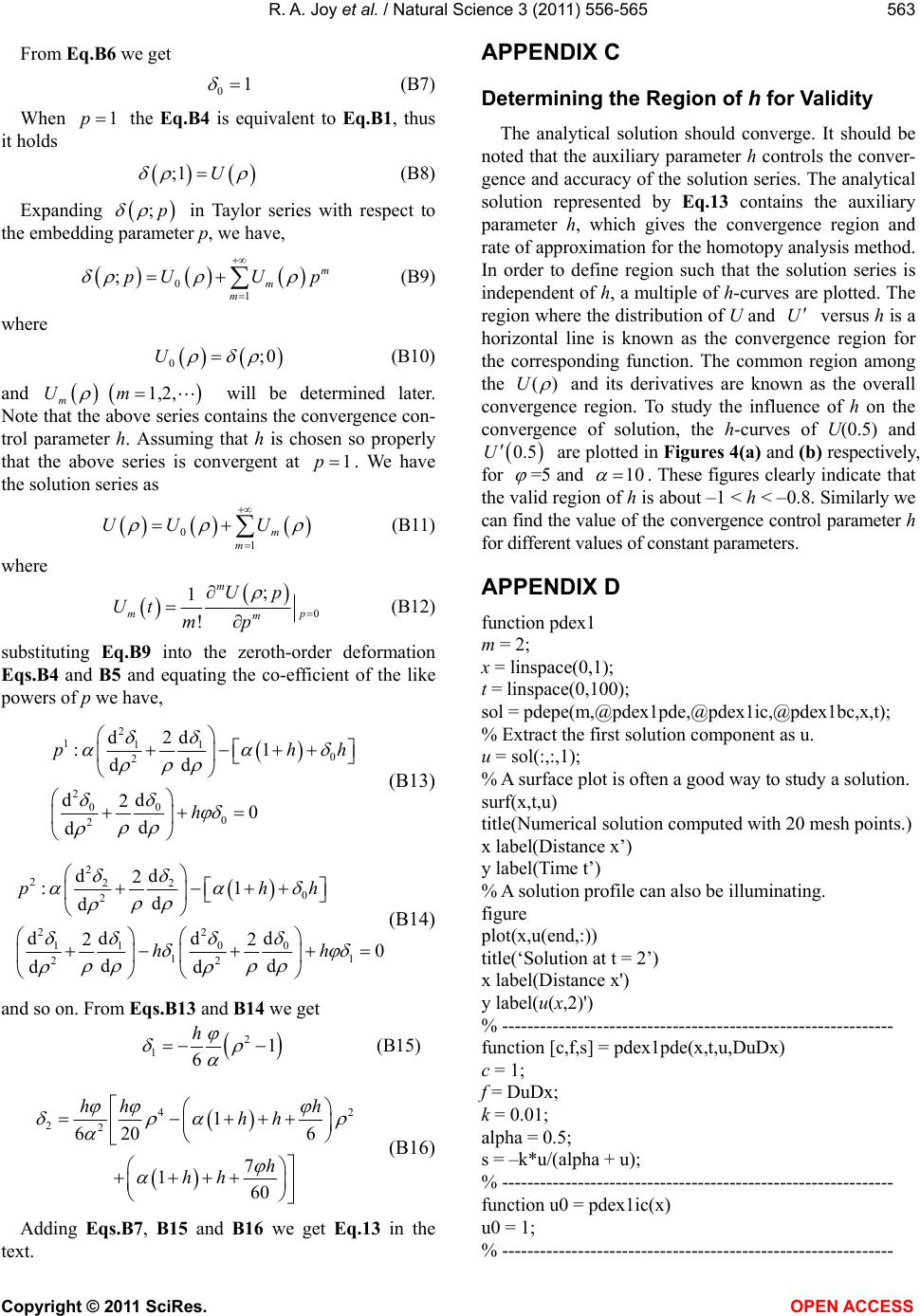
Figure 3. The normalized effectiveness factor η versus Thiele
moduilli φ for various values of parameter α. The curves are
plotted using Eq.13. Here h = –0.135.
effectiveness factor increases with increasing values of

.
6. CONCLUSIONS
A non-linear time independent equation has been
formulated and solved analytically using Homotopy
analysis method. The primary result of this work is the
first approximate calculations of substrate concentrations
and effectiveness factor for non-linear Michaelis-Menten
kinetic scheme. A simple closed form of analytical ex-
pressions of steady-state substrate and effectiveness fac-
tor are given. The analytical expressions for the substrate
concentration profiles for all values of parameters

and

are derived using Homotopy analysis method.
This method is an extremely simple method and it is also
a promising method to solve other non-linear equations.
The extension of this procedure to other direct reaction
of substrate at underlying microdisc electrode surface
seems possible.
7. ACKNOWLEDGEMENTS
This work was supported by the Department of Science and Tech-
nology (DST) Government of India. The authors also thank Mr.M.S.
Meenakshisundaram, Secretary, The Madura College Board, Principal
and S.Thiagarajan Head of the Department of Mathematics, The
Madura College, Madurai, India for their constant encouragement. It is
our pleasure to thank the referees for their valuable comments.
REFERENCES
[1] Gomez J.L, Bodalo A., Gomez E., Bastida J. and Maximo
M.F. (2003) Two-parameter model for evaluating effec-
tiveness factor for immobilized enzymes with reversible
Michaelis–Menten kinetics. Chemical Engineering Sci-
ence, 58, 4287-4290.
[2] Manjon A., Iborra J.L., Gomez J.L., Gomez E., Bastida J.
and Bodalo A. (1987) Evaluation of the effectiveness
factor along immobilized enzyme fixed-bed reactors:
Design of a reactor with naringinase covalently immo-
bilized into glycophase-coated porous glass. Biotech-
nology and Bioengineering, 30, 491-497.
doi:10.1002/bit.260300405
[3] Bodalo S.A., Gomez C.J.L., Gomez E., Bastida R.J. and
Martinez M. E. (1993) Transient stirred-tank reactors op-
erating with immobilized enzyme systems: Analysis and
simulation models and their experimental checking. Bio-
technology Progress, 9, 166-173.
doi:10.1021/bp00020a008
[4] Bodalo A., Gomez J.L., Gomez E., Bastida J. and
Maximo M.F. (1995) Fluidized bed reactors operating
with immobilized enzyme systems: Design model and its
experimental verification. Enzyme and Microbial Tech-
nology, 17, 915-922.
doi:10.1016/0141-0229(94)00125-B
[5] Carnahan B., Luther H.A. and Wilkes J.O. (1969) Ap-
plied numerical methods, Wiley, New York.
[6] Villadsen J., Michelsen M.L. (1978) Solution of differen-
tial equation models by polynomial approximation. New
York: Prentice-Hall, Englewood Cliffs.
[7] Lee J. and Kim D.H. (2005) An improved shooting
method for computation of effectiveness factors in po-
rous catalysts. Chemical Engineering Science, 60, 5569-
5573. doi:10.1016/j.ces.2005.05.027
[8] Lyons M.E.G., Greer J.C., Fitzgerald C.A., Bannon T.
and Bartlett P.N. (1996) Reaction/Diffusion with Micha-
elis- Menten kinetics in electroactive polymer films Part
1. The steady-state amperometric response. Analyst, 12,
1715.
[9] Lyons M.E.G., Bannon T., Hinds G. and Rebouillat S.
(1998) Reaction/Diffusion with Michaelis-Menten kinet-
ics in electroactive polymer films Part 1. The transient
amperometric response. Analyst, 123, 1947.
doi:10.1039/a803274b
[10] Lyons M.E.G., Murphy J., Bannon T. and Rebouillat S.
(1999) Reaction, diffusion and migration in conducting
polymer electrodes: Analysis of the steady-state am-
perometric response. Journal of Solid State Electrochem-
istry, 3, 154-162.
doi:10.1007/s100080050142
[11] Moo-Young M. and Kobayashi T. (1972) Effectiveness
factors for immobilized enzyme reactions. Canadian
Journal of Chemical Engineering, 50, 162-167.
doi:10.1002/cjce.5450500204
[12] Kobayashi T. and Laidler K. J. (1973) Effectiveness fac-
tor calculations for immobilized enzyme catalysts. Bio-
chimica et Biophysica Acta, 1, 302-311.
[13] Engasser J.M. and Horvath J.C. (1973) Metabolism:
interplay of membrane transport and consecutive en-
zymic reaction. Journal of Theoretical Biology, 42,
137-155. doi:10.1016/0022-5193(73)90153-7
[14] Marsh D.R., Lee Y.Y. and Tsao G.T. (1973) Immobilized
glucoamylase on porous glass. Biotechnology and Bio-
engineering, 15, 483-492. doi:10.1002/bit.260150305
[15] Hamilton B.K., Cardner C.R. and Colton C.K. (1974)
Effect of diffusional limitations on lineweaver-burk plots
for immobilized enzymes. AIChE Journal, 20, 503-510.

R. A. Joy et al. / Natural Science 3 (2011) 556-565 561
doi:10.1002/aic.690200310
[16] Rovito B.J. and Kittrell J.R. (1973) Film and pore diffu-
sion studies with immobilized glucose Oxidase. Bio-
technology and Bioengineering, 15, 143-161.
doi:10.1002/bit.260150111
[17] Engasser J.M. (1978) The experimental results accorded
quantitatively with the theory of diffusion limitation.
Biochimica et Biophysica Acta, 526, 301-310.
[18] Aydogan O., Bayraktar E. and Mehmetoglu U. (2011)
Determination of effective diffusion coefficient of ace-
tophenone in carrageenan and asymmetric bioreduction
in packed bed reactor. Journal of Molecular Catalysis B:
Enzymatic, 72, 46-52.
doi:10.1016/j.molcatb.2011.04.023
[19] Puida M., Malinauskas A., Ivanauskas F. (2011) Mode-
ling of electrocatalysis at conducting polymer modified
electrodes: Nonlinear current-concentration profiles. Jour-
nal of Mathematical chemistry, 49, 1151-1162.
doi:10.1007/s10910-011-9802-y
[20] Marc A. and Engasser J.M. (1982) Influence of substrate
and product diffusion on the heterogeneous kinetics of
enzymic reversible reactions. Journal of Theoretical Bi-
ology, 94, 179-189.
doi:10.1016/0022-5193(82)90339-3
[21] Goldman R., Keden O., Silman I.H., Caplan S.R. and
Katchalski E. (1968) Papain-collodion membranes. I.
Preparation and properties. Biochemistry, 7, 486-500.
doi:10.1021/bi00842a002
[22] Engasser J.M. and Horvath C. (1974) Inhibition of bound
enzymes. II. characterization of product inhibition and
accumulation. Biochemistry, 133, 849-3854.
[23] Ramachandran P.A. (1975) Solution of immobilized en-
zyme problems by collocation methods. Biotechnology
and Bioengineering, 17, 211-226.
doi:10.1002/bit.260170207
[24] Liao S.J. (1992) The proposed homotopy analysis tech-
nique for the solution of nonlinear problems, Ph. D. The-
sis, Shanghai Jiao Tong University, Shanghai.
[25] Awawdeh F., Jaradat H.M. and Alsayyed O. (2009)
Solving System of DAEs by Homotopy Analysis. Chaos
Solitons and Fractals, 42, 1422-1427.
doi:10.1016/j.chaos.2009.03.057
[26] Jafari H., Chun C., Seifi S. and Saeidy M., (2009) Ana-
lytical solution for nonlinear Gas Dynamic equation by
Homotopy Analysis Method. Applied Mathmatics, 4,
149-154.
[27] Sohouli A.R., Famouri M., Kimiaeifar A. and Domairry
G., (2010) Application of homotopy analysis method for
natural convection of Darcian fluid about a vertical full
cone embedded in pours media prescribed surface heat
flux. Communications in Nonlinear Science and Nu-
merical Simulation, 15, 1691-1699.
doi:10.1016/j.cnsns.2009.07.015
[28] Domairry G. and Fazeli M. (2009) Homotopy analysis
method to determine the fin efficiency of convective
straight fins with temperature-dependent thermal con-
ductivity. Communications in Nonlinear Science and
Numerical Simulation, 14, 489-499.
doi:10.1016/j.cnsns.2007.09.007
[29] Liao S.J. (2004) On the homotopy analysis method for
nonlinear problems. Applied Mathematics and Computa-
tion, 147, 499-513.
doi:10.1016/S0096-3003(02)00790-7
[30] Domairry G. and Bararnia H. (2008) An Approximation
of the Analytic Solution of Some Nonlinear Heat Trans-
fer Equations: A Survey by using Homotopy Analysis
Method. Advanced studies in Theoretical Physics, 2,
507-518.
[31] Liao S.J. (2003) Beyond Perturbation: Introduction to the
Homotopy analysis method. Chapman and Hall, CRC
Press, Boca Raton. doi:10.1201/9780203491164

R. A. Joy et al. / Natural Science 3 (2011) 556-565 562
APPENDIX A
Basic Idea of Liao’s [31] Homotopy Analysis
method
Consider the following differential Eq.31:

0Nut 
 (A1)
where, Ν is a nonlinear operator, t denotes an independ-
ent variable, u(t) is an unknown function. For simplicity,
we ignore all boundary or initial conditions, which can
be treated in the similar way. By means of generalizing
the conventional homotopy method, Liao constructed the
so-called zero-order deformation equation as:

0
1; ;pLtpu tphHtNtp   

(A2)
where


0,1p is the embedding parameter, h ≠ 0 is a
nonzero auxiliary parameter, H(t) ≠ 0 is an auxiliary
function, L is an auxiliary linear operator,


0
ut
is an
initial guess of u(t) and

:tp 
is an unknown func-
tion. It is important, that one has great freedom to choose
auxiliary unknowns in HAM. Obviously, when 0p

and 1p, it holds:
 
0
;0tut  and
 
;1tut   (A3)
respectively. Thus, as p increases from 0 to 1, the solu-
tion

;tp  varies from the initial guess

0
ut to the
solution

ut . Expanding

;tp  in Taylor series
with respect to p, we have:
 
0
1
;m
m
m
tputut p 



 (A4)
where
 
0
;
1
!
m
mp
m
tp
ut mp



 (A5)
If the auxiliary linear operator, the initial guess, the
auxiliary parameter h, and the auxiliary function are so
properly chosen, the series Eq.A4 converges at p =1
then we have:
 
0
1
m
m
utu tut



. (A6)
Define the vector

01
,, ,
nn
uu uu (A7)
Differentiating Eq.A2 for m times with respect to the
embedding parameter p, and then setting p = 0 and fi-
nally dividing them by m!, we will have the so-called
mth-order deformation equation as:


 
11mmm mm
LuuhH t 

u (A8)
where



1
10
1
;
1
1!
m
mm p
m
Ntp
mp









u (A9)
and
0, 1,
1, 1.
m
m
m




 (A10)
Applying 1
L

on both side of Eq.A8 , we get



 
1
11 mmm mm
ututhL Ht 


  

u (A11)
In this way, it is easy to obtain m u for 1,m at
th
M
order, we have
 
0
M
m
m
utu t

 (A12)
when M, we get an accurate approximation of
the original Eq.A1 . For the convergence of the above
method we refer the reader to Liao [31]. If Eq. A1 admits
unique solution, then this method will produce the
unique solution. If Eq.A1 does not possess unique solu-
tion, the HAM will give a solution among many other
(possible) solutions.
APPENDIX B
2
2
1d d
dd
UU
U







 (B1)
Now the boundary conditions become
d
0,0
d
U


 (B2)
1, 1U


 (B3)
In order to solve Eq.B1 by means of the HAM, we
first construct the Zeroth-order deformation equation by
taking


1Ht

,


2
2
2
2
d2d
1d
d
d2d
d
d
p
ph




 








 





(B4)
subject to the boundary conditions


0; 0p 
,


1; 1p   (B5)
where


0, 1p is an embedding parameter and h ≠ 0
is the so-called convergence control parameter. When
0p



2
2
d;0 d;0
20
d d
 


 (B6)

R. A. Joy et al. / Natural Science 3 (2011) 556-565 563
From Eq.B6 we get
01


(B7)
When 1p the Eq. B4 is equivalent to Eq.B1, thus
it holds



;1 U

  (B8)
Expanding

;p 
in Taylor series with respect to
the embedding parameter p, we have,
 
0
1
;m
m
m
pUU p  



 (B9)
where



0;0U
  (B10)
and


m
U


1,2, m will be determined later.
Note that the above series contains the convergence con-
trol parameter h. Assuming that h is chosen so properly
that the above series is convergent at 1p. We have
the solution series as
 
0
1
m
m
UU U





 (B11)
where



0
;
1
!
m
mp
m
Up
Ut mp



 (B12)
substituting Eq .B 9 into the zeroth-order deformation
Eqs.B4 and B5 and equating the co-efficient of the like
powers of p we have,

2
111
0
2
2
00
0
2
dd
2
:1
d d
dd
20
d d
phh
h


 


 












(B13)

2
222
0
2
2 2
00 11
11
22
dd 2
:1
d
d
dd dd 22
0
dd dd
phh
hh




 

  

 



 
 
 
 
(B14)
and so on. From Eqs.B13 and B14 we get

2
11
6
h 


 (B15)


42
221
20 6 6
7
160
hh h
hh
h
hh



















(B16)
Adding Eqs.B7 , B15 and B1 6 we get Eq.13 in the
text.
APPENDIX C
Determining the Region of h for Validity
The analytical solution should converge. It should be
noted that the auxiliary parameter h controls the conver-
gence and accuracy of the solution series. The analytical
solution represented by Eq.13 contains the auxiliary
parameter h, which gives the convergence region and
rate of approximation for the homotopy analysis method.
In order to define region such that the solution series is
independent of h, a multiple of h-curves are plotted. The
region where the distribution of U and U versus h is a
horizontal line is known as the convergence region for
the corresponding function. The common region among
the )(

U and its derivatives are known as the overall
convergence region. To study the influence of h on the
convergence of solution, the h-curves of U(0.5) and


0.5U are plotted in Figures 4(a) and (b) respectively,
for

=5 and 10


. These figures clearly indicate that
the valid region of h is about –1 < h < –0.8. Similarly we
can find the value of the convergence control parameter h
for different values of constant parameters.
APPENDIX D
function pdex1
m = 2;
x = linspace(0,1);
t = linspace(0,100);
sol = pdepe(m,@pdex1pde,@pdex1ic,@pdex1bc,x,t);
% Extract the first solution component as u.
u = sol(:,:,1);
% A surface plot is often a good way to study a solution.
surf(x,t,u)
title(Numerical solution computed with 20 mesh points.)
x label(Distance x’)
y label(Time t’)
% A solution profile can also be illuminating.
figure
plot(x,u(end,:))
title(‘Solution at t = 2’)
x label(Distance x')
y label(u(x,2)')
% --------------------------------------------------------------
function [c,f,s] = pdex1pde(x,t,u,DuDx)
c = 1;
f = DuDx;
k = 0.01;
alpha = 0.5;
s = –k*u/(alpha + u);
% --------------------------------------------------------------
function u0 = pdex1ic(x)
u0 = 1;
% --------------------------------------------------------------

R. A. Joy et al. / Natural Science 3 (2011) 556-565 564
function [pl,ql,pr,qr] = pdex1bc(xl,ul,xr,ur,t)
pl = 0;
ql = 1;
pr = ur–1;
qr = 0;
APPENDIX E
Consider
U
d
dU
d
d














2
2
1 (E1)
(a)
(b)
Figure 4. The h curves to indicate the convergence region, for
φ = 5 and α = 10.
Boundary conditions are:
.0 ;0
,1 U;1






d
dU (E2)
Using reduction of order, we have
2; ; 0.PQ R 



(E3)
Let
Uuv (E4)
Substitute Eq.E4 in Eq.E1 and choose u such that
d
20
d
uPu



Substituting the value of P, we obtain
1
u


(E5)
Now the Eq.E1 reduces to
11
vQvR



 (E6)
2
11
1d
Q, 0
2d 4
PR
QR
u



  (E7)
Substituting Eq.E7 in Eq.E6 we obtain
0.vv




 (E8)
Solving we obtain
AeBe- .v




 (E9)
Substituting Eq.E5 and Eq.E9 in Eq.E4 we have
1AeBe- U









(E10)
Using the boundary conditions we obtain the value of
the constants as
11
; B
2sinh 2sinh
A





 
 
 
 
(E11)
Substituting in Eq.E10 we obtain the solution as
sinh
sinh
U














(E12)

R. A. Joy et al. / Natural Science 3 (2011) 556-565 565
Appendix F
Nomenclature and Units
Symbols
S
C Concentration of the substrate (mol·cm–3)
P
C Concentration of the product (mol·cm–3)
r Radial co-ordinate (cm)
SR
C Local substrate concentration (mol·cm–3)
P
R
C Local product concentration (mol·cm–3)
eq
K
Reaction equilibrium constant (none)
m
K
Michaelis-Menten constant (mol·cm–3)
S
D
Diffusion coefficient of the substrate (cm2·sec–1)
P
D
Diffusion coefficient of the product (cm2·sec–1)
R Radius of the particle (cm)
S
V Local reaction rate per unit of catalytic particle volume
(mol·cm–3·s–1)
m
V Maximum reaction rate per unit of catalytic particle
volume (mol·cm–3·s–1)
U Normalized substrate concentration (none)
,

 Normalized Thiele modulus (none)

Effectiveness factor (none)