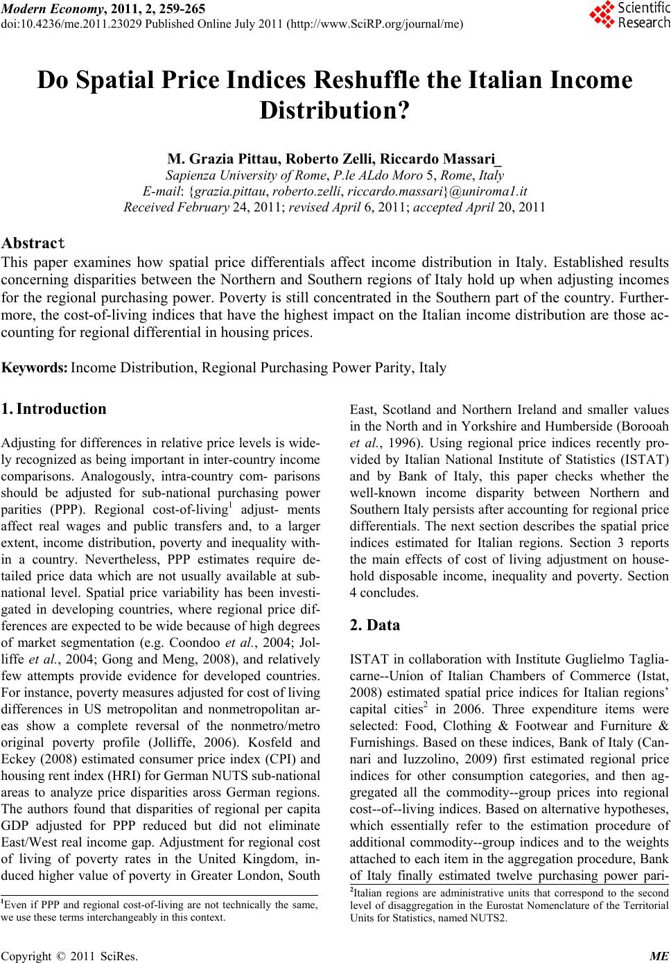Modern Economy, 2011, 2, 259-265
doi:10.4236/me.2011.23029 Published Online July 2011 (http://www.SciRP.org/journal/me)
Do Spatial Price Indices Reshuffle the Italian Income
Distribution?
M. Grazia Pittau, Roberto Zelli, Riccardo Massari_
Sapienza University of Rome, P.le ALdo Moro 5, Rome, Italy
Received February 24 , 20 1 1; revised April 6, 2011; acce pte d April 20, 2011
Abstract
This paper examines how spatial price differentials affect income distribution in Italy. Established results
concerning disparities between the Northern and Southern regions of Italy hold up when adjusting incomes
for the regional purchasing power. Poverty is still concentrated in the Southern part of the country. Further-
more, the cost-of-living indices that have the highest impact on the Italian income distribution are those ac-
counting for regional differential in housing prices.
Keywords: Income Distribution, Regional Purchasing Power Parity, Italy
1. Introduction
Adjusting for differences in relative price levels is wide-
ly recognized as being important in inter-country inco me
comparisons. Analogously, intra-country com- parisons
should be adjusted for sub-national purchasing power
parities (PPP). Regional cost-of-living1 adjust- ments
affect real wages and public transfers and, to a larger
extent, income distribution, poverty and inequality with-
in a country. Nevertheless, PPP estimates require de-
tailed price data which are not usually available at sub-
national level. Spatial price variability has been investi-
gated in developing countries, where regional price dif-
ferences are expected to be wide because of high degrees
of market segmentation (e.g. Coondoo et al., 2004; Jol-
liffe et al., 2004; Gong and Meng, 2008), and relatively
few attempts provide evidence for developed countries.
For instance, poverty measures adjusted for cost of living
differences in US metropolitan and nonmetropolitan ar-
eas show a complete reversal of the nonmetro/metro
original poverty profile (Jolliffe, 2006). Kosfeld and
Eckey (2008) estimated consumer price index (CPI) and
housing rent i n dex ( HR I) for German NUTS sub-national
areas to analyze price disparities aross German regions.
The authors found that disparities of regional per capita
GDP adjusted for PPP reduced but did not eliminate
East/West real income gap. Adjustment for regional cost
of living of poverty rates in the United Kingdom, in-
duced higher value of poverty in Greater London, South
East, Scotland and Northern Ireland and smaller values
in the North and in Yor kshire and Humberside (Borooah
et al., 1996). Using regional price indices recently pro-
vided by Italian National Institute of Statistics (ISTAT)
and by Bank of Italy, this paper checks whether the
well-known income disparity between Northern and
Southern Italy persists after accounting for regional price
differentials. The next section describes the spatial price
indices estimated for Italian regions. Section 3 reports
the main effects of cost of living adjustment on house-
hold disposable income, inequality and poverty. Section
4 concludes.
2. Data
ISTAT in collaboration with Institute Guglielmo Taglia-
carne--Union of Italian Chambers of Commerce (Istat,
2008) estimated spatial price indices for Italian regions’
capital cities2 in 2006. Three expenditure items were
selected: Food, Clothing & Footwear and Furniture &
Furnishings. Based on these indices, Bank of Italy (Can-
nari and Iuzzolino, 2009) first estimated regional price
indices for other consumption categories, and then ag-
gregated all the commodity--group prices into regional
cost--of--living ind ices. Based on alternative hypotheses,
which essentially refer to the estimation procedure of
additional commodity--group indices and to the weights
attached to each item in the aggregation pr ocedure, Bank
of Italy finally estimated twelve purchasing power pari-
2Italian regions are administrative units that correspond to the second
level of disaggregation in the Eurostat Nomenclature of the Territorial
Units for Statistics, named NUTS2.
1Even if PPP and regional cost-of-living are not technically the same,
we use these terms interchangeably in this context.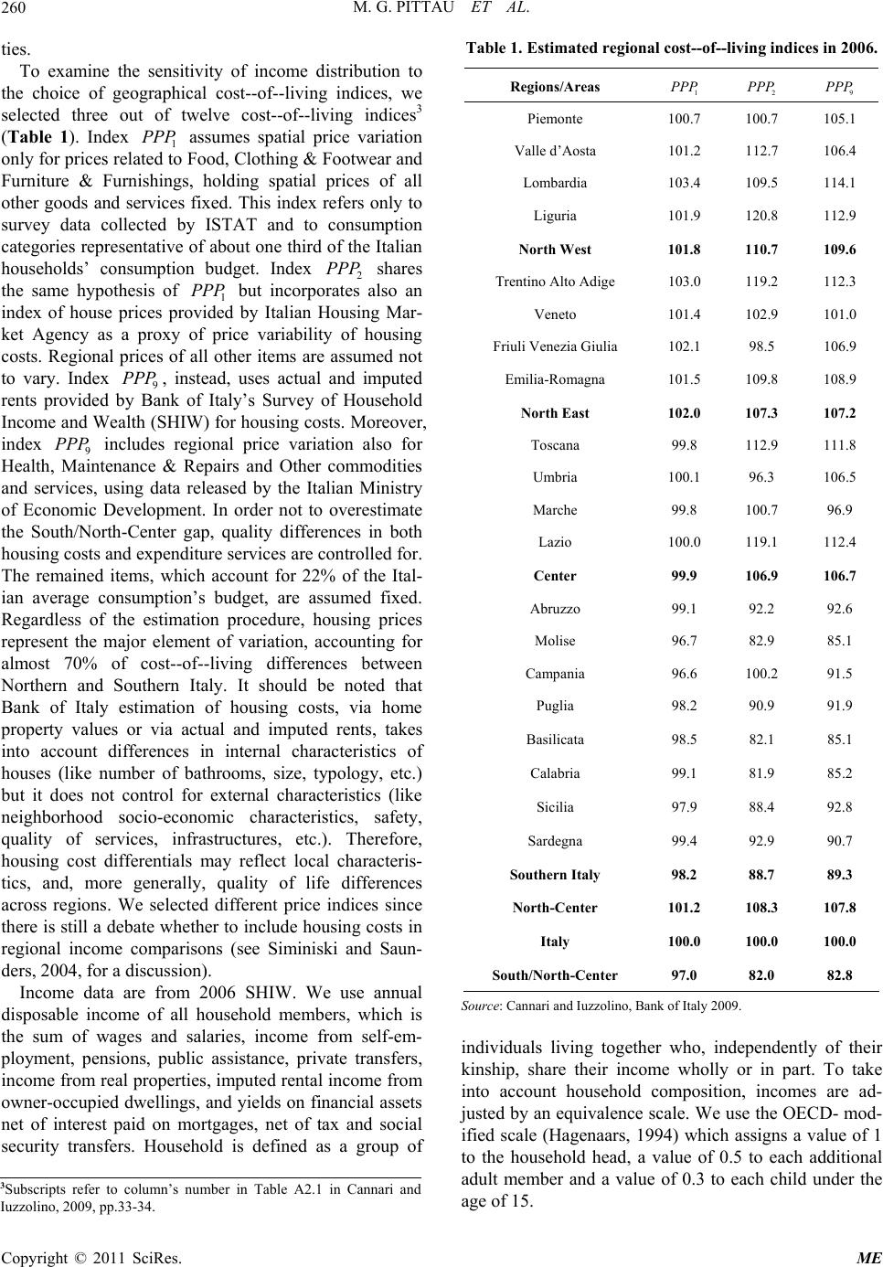

M. G. PITTAU ET AL. 260
ties.
To examine the sensitivity of income distribution to
the choice of geographical cost--of--living indices, we
selected three out of twelve cost--of--living indices3
(Table 1). Index 1 assumes spatial price variation
only for prices related to Food, Clothing & Footwear and
Furniture & Furnishings, holding spatial prices of all
other goods and services fixed. This index refers only to
survey data collected by ISTAT and to consumption
categories representative of about one third of the Italian
households’ consumption budget. Index 2 shares
the same hypothesis of 1 but incorporates also an
index of house prices provided by Italian Housing Mar-
ket Agency as a proxy of price variability of housing
costs. Regional prices of all other items are assumed not
to vary. Index 9, instead, uses actual and imputed
rents provided by Bank of Italy’s Survey of Household
Income and Wealth (SHIW) for housing costs. Moreover,
index 9 includes regional price variation also for
Health, Maintenance & Repairs and Other commodities
and services, using data released by the Italian Ministry
of Economic Development. In order not to overestimate
the South/North-Center gap, quality differences in both
housing costs and expenditure services are controlled for.
The remained items, which account for 22% of the Ital-
ian average consumption’s budget, are assumed fixed.
Regardless of the estimation procedure, housing prices
represent the major element of variation, accounting for
almost 70% of cost--of--living differences between
Northern and Southern Italy. It should be noted that
Bank of Italy estimation of housing costs, via home
property values or via actual and imputed rents, takes
into account differences in internal characteristics of
houses (like number of bathrooms, size, typology, etc.)
but it does not control for external characteristics (like
neighborhood socio-economic characteristics, safety,
quality of services, infrastructures, etc.). Therefore,
housing cost differentials may reflect local characteris-
tics, and, more generally, quality of life differences
across regions. We selected different price indices since
there is still a debate whether to in clude housing costs in
regional income comparisons (see Siminiski and Saun-
ders, 2004, f or a discussion).
PPP
PPP
PPP
PPP
PPP
Income data are from 2006 SHIW. We use annual
disposable income of all household members, which is
the sum of wages and salaries, income from self-em-
ployment, pensions, public assistance, private transfers,
income from real properties, imputed rental income from
owner-occupied dwelling s, and yields on financial assets
net of interest paid on mortgages, net of tax and social
security transfers. Household is defined as a group of
Table 1. Estimated regional cost--of--living indices in 2006.
Regions/Areas 1
PPP 2 PPP 9 PPP
Piemonte 100.7 100.7 105.1
Valle d’Aosta 101.2 112.7 106.4
Lombardia 103.4 109.5 114.1
Liguria 101.9 120.8 112.9
North West 101.8 110.7 109.6
Trentino Alto Adige 103.0 119.2 112.3
Veneto 101.4 102.9 101.0
Friuli Venezia Giulia 102.1 98.5 106.9
Emilia-Romagna 101.5 109.8 108.9
North East 102.0 107.3 107.2
Toscana 99.8 112.9 111.8
Umbria 100.1 96.3 106.5
Marche 99.8 100.7 96.9
Lazio 100.0 119.1 112.4
Center 99.9 106.9 106.7
Abruzzo 99.1 92.2 92.6
Molise 96.7 82.9 85.1
Campania 96.6 100.2 91.5
Puglia 98.2 90.9 91.9
Basilicata 98.5 82.1 85.1
Calabria 99.1 81.9 85.2
Sicilia 97.9 88.4 92.8
Sardegna 99.4 92.9 90.7
Southern Italy 98.2 88.7 89.3
North-Center 101.2 108.3 107.8
Italy 100.0 100.0 100.0
South/North-Center 97.0 82.0 82.8
Source: Cannari and I u zzolino, Bank of Ita ly 2009.
individuals living together who, independently of their
kinship, share their income wholly or in part. To take
into account household composition, incomes are ad-
justed by an equivalence scale. We use the OECD- mod-
ified scale (Hagenaars, 1994) which assigns a value of 1
to the household head, a value of 0.5 to each additional
adult member and a value of 0.3 to each child under the
age of 15.
3Subscripts refer to column’s number in Table A2.1 in Cannari and
Iuzzolino, 2009, pp.33-34.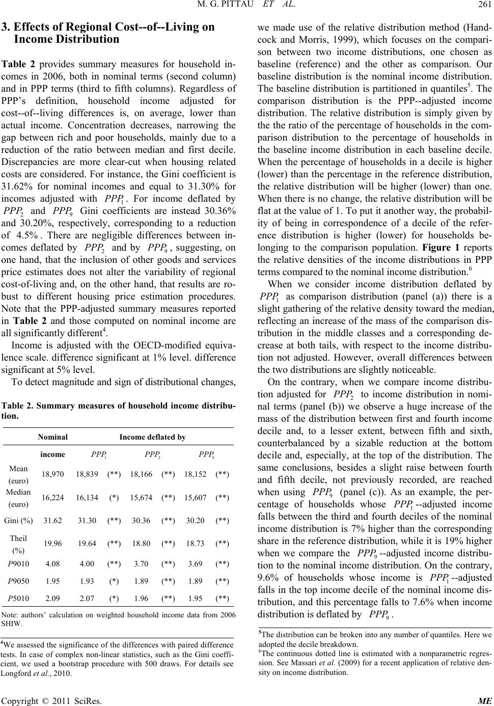

M. G. PITTAU ET AL.261
3. Effects of Regional Cost--of--Living on
Income Distribution
Table 2 provides summary measures for household in-
comes in 2006, both in nominal terms (second column)
and in PPP terms (third to fifth columns). Regardless of
PPP’s definition, household income adjusted for
cost--of--living differences is, on average, lower than
actual income. Concentration decreases, narrowing the
gap between rich and poor households, mainly due to a
reduction of the ratio between median and first decile.
Discrepancies are more clear-cut when housing related
costs are considered. For instance, the Gini coefficient is
31.62% for nominal incomes and equal to 31.30% for
incomes adjusted with 1. For income deflated by
2 and 9 Gini coefficients are instead 30.36%
and 30.20%, respectively, corresponding to a reduction
of . There are negligible differences between in-
comes deflated by 2 and by 9, suggesting, on
one hand, that the inclusion of other goods and services
price estimates does not alter the variability of regional
cost-of-living and, on the other hand, that results are ro-
bust to different housing price estimation procedures.
Note that the PPP-adjusted summary measures reported
in Table 2 and those computed on nominal income are
all significantly different4.
PPP
P
PPP
4.5%
PPP
PP PPP
Income is adjusted with the OECD-modified equiva-
lence scale. difference significant at 1% level. difference
significant at 5% level.
To detect magnitude and sign of distributional changes,
Table 2. Summary measures of household income distribu-
tion.
Nominal Income deflated by
income 1 PPP 2 PPP 9 PPP
Mean
(
euro
)
18,970 18,839 (**) 18,166 (**) 18,152(**)
Median
(
euro
)
16,224 16,134 (*) 15,674 (**) 15,607 (**)
Gini (%) 31.62 31.30 (**) 30.36 (**) 30.20(**)
Theil
(
%
)
19.96 19.64 (**) 18.80 (**) 18.73(**)
9010P 4.08 4.00 (**) 3.70 (**) 3.69 (**)
9050P 1.95 1.93 (*) 1.89 (**) 1.89 (**)
5010P 2.09 2.07 (*) 1.96 (**) 1.95 (**)
Note: authors’ calculation on weighted household income data from 2006
SHIW.
we made use of the relative distribution method (Hand-
cock and Morris, 1999), which focuses on the compari-
son between two income distributions, one chosen as
baseline (reference) and the other as comparison. Our
baseline distribution is the nominal income distribution.
The baseline distribution is partition ed in quantiles5. The
comparison distribution is the PPP--adjusted income
distribution. The relative distribution is simply given by
the the ratio of the percentage of househo lds in the com-
parison distribution to the percentage of households in
the baseline income distribution in each baseline decile.
When the percentage of households in a decile is higher
(lower) than the percentage in the reference distribution,
the relative distribution will be higher (lower) than one.
When there is no change, the relativ e distribution will be
flat at the value of 1. To put it another way, the probabil-
ity of being in correspondence of a decile of the refer-
ence distribution is higher (lower) for households be-
longing to the comparison population. Figure 1 reports
the relative densities of the income distributions in PPP
terms compared to the nominal income distribution.6
When we consider income distribution deflated by
1 as comparison distribution (panel (a)) there is a
slight gathering of the relative density toward the median,
reflecting an increase of the mass of the comparison dis-
tribution in the middle classes and a corresponding de-
crease at both tails, with respect to the income distribu-
tion not adjusted. However, overall differences between
the two distributions are slightly noticeable.
PPP
On the contrary, when we compare income distribu-
tion adjusted for 2 to income distribution in nomi-
nal terms (panel (b)) we observe a huge increase of the
mass of the distribution between first and fourth income
decile and, to a lesser extent, between fifth and sixth,
counterbalanced by a sizable reduction at the bottom
decile and, especially, at the top of the distribution. The
same conclusions, besides a slight raise between fourth
and fifth decile, not previously recorded, are reached
when using 9 (panel (c)). As an example, the per-
centage of households whose 1--adjusted income
falls between the third and fourth deciles of the nominal
income distribution is 7% higher than the corresponding
share in the reference distribution, wh ile it is 19% higher
when we compare the 9--adjusted income distribu-
tion to the nominal income distribution. On the con trary,
9.6% of households whose income is 1--adjusted
falls in the top income decile of the nominal income dis-
tribution, and this percentage falls to 7.6% when income
distribution is deflated by .
PPP
PPP PPP
PPP
PP
PPP
9
P
5The distribution can be broken into any number of quantiles. Here we
adopted the decile breakdown.
6The continuous dotted line is estimated with a nonparametric regres-
sion. See Massari et al. (2009) for a recent application of relative den-
sit
y
on income distribution.
4We assessed the significance of the differences with paired difference
tests. In case of complex non-linear statistics, such as the Gini coeffi-
cient, we used a bootstrap procedure with 500 draws. For details see
Longford et al., 2010.

M. G. PITTAU ET AL. 262
Figure 1. Relative distribution. The y-axis measures the relative fraction of households ranked by PPP adjusted income
distributions that falls in each nominal income distribution decile.
To observe what happens in terms of inequality and
poverty between and within Italian regions before and
after price-adjustment, we consider only 1 and
9, since the results obtained with largely
overlap those achieved with .
PPP
2
PPPP PP
poverty in Southern Italy (South and Islands) which is
not fully counterbalanced by households
at-risk-of-poverty in North-West and Central Italy. After
adjusting for 9, however, households
at-risk-of-poverty are still concentrated in Southern Italy
(almost 60% with respect to 68% in the no minal scale).
PPP
9
First, the decomposition of Theil index into be-
tween-region and within-region, reported in Table 3,
reveals a significant reduction in the between-region
component when PPP-adjusted income is accounted for.
Thus, since the within-region component remains stable6
the percentage contribution of the between-region com-
ponent drops from 14.4% for nominal income to 8.1%
for income -adjusted.
PPP
We now analyze how mean income changes in each
region when income is deflated by 1 (Figure 2(a))
or by 9 (Figure 2(b)). The magnitude of percent-
age changes is displayed with varying degree of gray.
The lighter (darker) the color, the higher is the increase
(decrease) of regional mean income after controlling for
regional PPP’s. The evidence in Figure 2(a) is rather
mixed, with positive changes mainly concentrated in the
Southern Italy, but with different degrees. Only Cam-
pania and Molise experience a percentage change higher
than . In the North-Central Italy, Tuscany and
Marche display positive changes of mean income, while
for the remaining regions we observe a decrease of the
mean, which ranges to very low values (Umbria and La-
zio), to a reduction of in Lombardy.
PPP
PPP
3%
3%
9
The percentage of households at-risk-of-poverty in
NUTS1 macro-areas is reported in Table 4. Households
at-risk-of-poverty are those below a low-income thresh-
old, which is defined as 60 per cent of the median
equivalent income. The overall percentage of households
at risk of poverty decreases from 18% to 15.7%. This
reduction is due to a significant decrease of the rate of
PPP
Table 3. Decomposition of Theil index between and within
regions. Estimated values and percentage contribution. Results are more definite in Figure 2(b), with a po-
larization between Southern regions which display an
increase higher than , and North-Central regions that
experience a decline in mean income of over , with
the exception of Veneto (
3% 3%
1%

).
Income Theil Between Within Between Within
index component component % contribution
Nominal 19.96 2.88 17.08 14.4 85.6
1-
deflated
PPP 19.64 2.55 17.09 13.0 87.0
9-
deflated
PPP 18.73 1.51 17.22 8.1 91.9
Finally, Figure 3 reports the relative distribution of
households living in North-Central Italy (comparison
distribution) with respect to the distribution of those liv-
ing in Southern Italy (reference distribution), according
to different deflation adjustments. The gap between
North-Central and Southern Italy reduces, after adjusting
with 9, but remains wide. For a household living in
North-Central Italy the probability of falling between
PPP
6Small differences in the within-regions component are d ue to small changes
in the income shares of the regions us ed as weights in computing the com-
ponent.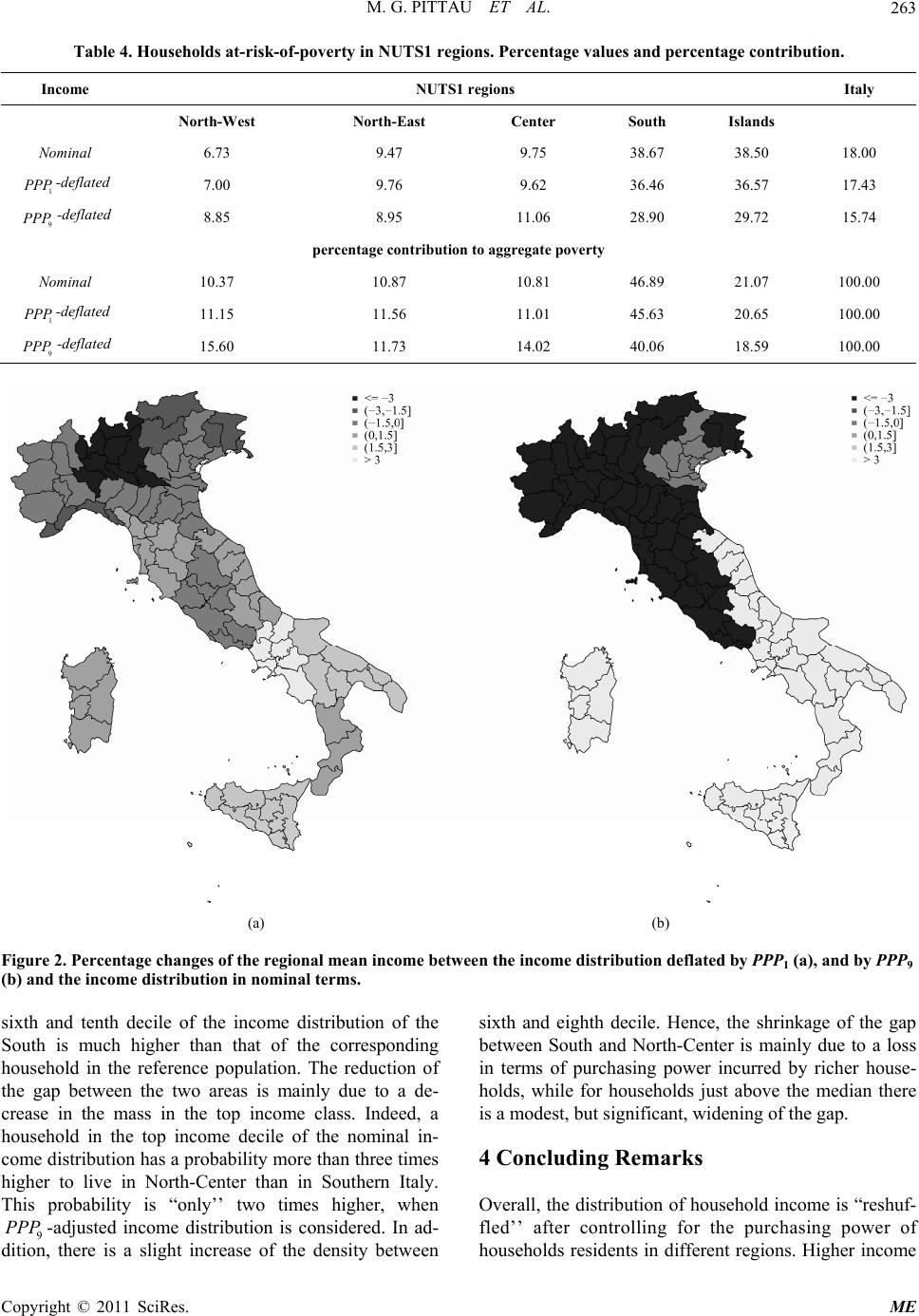

M. G. PITTAU ET AL.263
Table 4. Households at-risk-of-poverty in NUTS1 regions. Percentage values and percentage contribution.
Income NUTS1 regions Italy
North-West North-East Center South Islands
Nominal 6.73 9.47 9.75 38.67 38.50 18.00
1
PPP -deflated 7.00 9.76 9.62 36.46 36.57 17.43
9
PPP -deflated 8.85 8.95 11.06 28.90 29.72 15.74
percentage contribution to aggregate poverty
Nominal 10.37 10.87 10.81 46.89 21.07 100.00
1
PPP -deflated 11.15 11.56 11.01 45.63 20.65 100.00
9
PPP -deflated 15.60 11.73 14.02 40.06 18.59 100.00
(a) (b)
Figure 2. Percentage changes of the regional mean income between the income distribution deflated by PPP1 (a), and by PPP9
(b) and the income distribution in nominal terms.
sixth and tenth decile of the income distribution of the
South is much higher than that of the corresponding
household in the reference population. The reduction of
the gap between the two areas is mainly due to a de-
crease in the mass in the top income class. Indeed, a
household in the top income decile of the nominal in-
come distribution has a pro bability more than three times
higher to live in North-Center than in Southern Italy.
This probability is “only’’ two times higher, when
9-adjusted income distribution is considered. In ad-
dition, there is a slight increase of the density between
sixth and eighth decile. Hence, the shrinkage of the gap
between South and North-Center is mainly due to a loss
in terms of purchasing power incurred by richer house-
holds, while for households just above the median there
is a modest, but significant, widening of the gap.
PPP
4 Concluding Remarks
Overall, the distribution of household income is “reshuf-
fled’’ after controlling for the purchasing power of
households residents in different regions. Higher income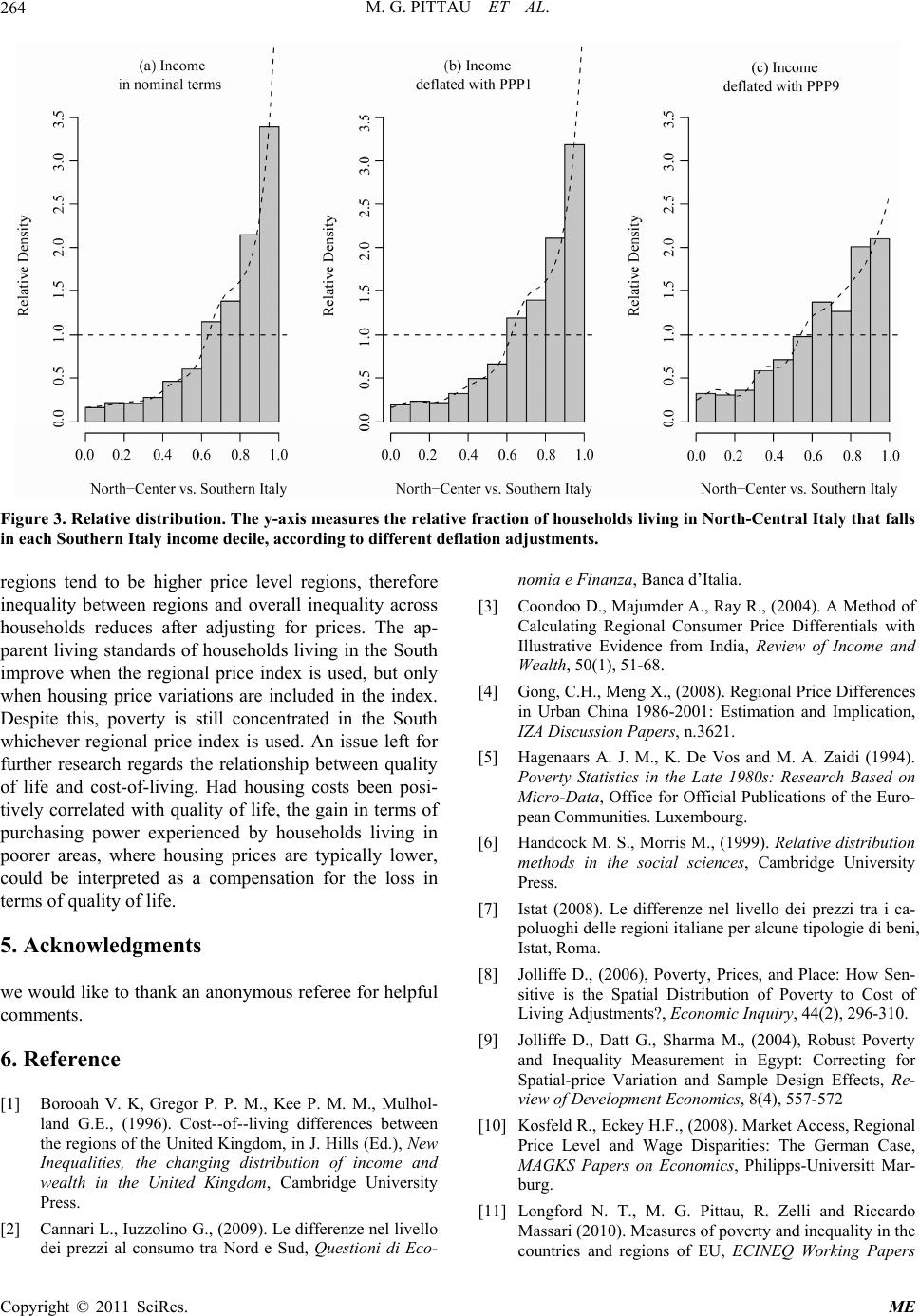

M. G. PITTAU ET AL. 264
Figure 3. Relative distribution. The y-axis measures the relative fraction of households living in North-Central Italy that falls
in each Southern Italy income decile, according to different deflation adjustments.
regions tend to be higher price level regions, therefore
inequality between regions and overall inequality across
households reduces after adjusting for prices. The ap-
parent living standards of households living in the South
improve when the regional price index is used, but only
when housing price variations are included in the index.
Despite this, poverty is still concentrated in the South
whichever regional price index is used. An issue left for
further research regards the relationship between quality
of life and cost-of-living. Had housing costs been posi-
tively correlated with quality of life, the gain in terms of
purchasing power experienced by households living in
poorer areas, where housing prices are typically lower,
could be interpreted as a compensation for the loss in
terms of quality of life.
5. Acknowledgments
we would like to thank an anonymous referee for helpful
comments.
6. Reference
[1] Borooah V. K, Gregor P. P. M., Kee P. M. M., Mulhol-
land G.E., (1996). Cost--of--living differences between
the regions of the United Kingdom, in J. Hills (Ed.), New
Inequalities, the changing distribution of income and
wealth in the United Kingdom, Cambridge University
Press.
[2] Cannari L., Iuzzolino G., (2009). Le differenze nel livello
dei prezzi al consumo tra Nord e Sud, Questioni di Eco-
nomia e Finanza, Banca d’Italia.
[3] Coondoo D., Majumder A., Ray R., (2004). A Method of
Calculating Regional Consumer Price Differentials with
Illustrative Evidence from India, Review of Income and
Wealth, 50(1), 51-68.
[4] Gong, C.H., Meng X., (2008). Regional Price Differences
in Urban China 1986-2001: Estimation and Implication,
IZA Discussion Papers, n.3621.
[5] Hagenaars A. J. M., K. De Vos and M. A. Zaidi (1994).
Poverty Statistics in the Late 1980s: Research Based on
Micro-Data, Office for Official Publications of the Euro-
pean Communities. Luxembourg.
[6] Handcock M. S., Morris M., (1999). Relative distribution
methods in the social sciences, Cambridge University
Press.
[7] Istat (2008). Le differenze nel livello dei prezzi tra i ca-
poluoghi delle regioni italiane per alcune tipologie di beni,
Istat, Roma.
[8] Jolliffe D., (2006), Poverty, Prices, and Place: How Sen-
sitive is the Spatial Distribution of Poverty to Cost of
Living Adjustments?, Economic Inquiry, 44(2), 296-310.
[9] Jolliffe D., Datt G., Sharma M., (2004), Robust Poverty
and Inequality Measurement in Egypt: Correcting for
Spatial-price Variation and Sample Design Effects, Re-
view of Development Economics, 8(4), 557-572
[10] Kosfeld R., Eckey H.F., (2008). Market Access, Regional
Price Level and Wage Disparities: The German Case,
MAGKS Papers on Economics, Philipps-Universitt Mar-
burg.
[11] Longford N. T., M. G. Pittau, R. Zelli and Riccardo
Massari (2010). Measures of poverty and inequality in the
countries and regions of EU, ECINEQ Working Papers

M. G. PITTAU ET AL.265
182, Society f or th e S tu dy of Economic Inequality .
[12] Massari R., M. G. Pittau and R. Zelli (2009). A dwindling
middle class? Italian evidence in the 2000s. Journal of
Economic Inequality, 7(4), pages 333-350.
[13] Siminski P. and P. Saunders (2004). Accounting for
Housing Costs in Regional Income Comparisons. Aus-
tralasian Journal of Regional Studies 10(2), 139-156.