 Modern Economy, 2011, 2, 354-370 doi:10.4236/me.2011.23039 Published Online July 2011 (http://www.SciRP.org/journal/me) Copyright © 2011 SciRes. ME Foreign Exchange Reserves Demand Model Based on Chinese Government Utility Maximization and Analysis of Chinese Fore ign Exchange Reserves* Shihong Zeng School of Economics & Management, Beijing University of Technology, Beijing, China E-mail: zengshihong2000@yahoo.com.cn Received April 15, 2011; revised April 25, 2011; accepted June 3, 2011 Abstract At the end of 2010 China’s foreign exchange reserve reached $2847.34 billion, the author designs the maxi- mum government utility function when consider the China government buys a part foreign exchange if company earns, it means that the China government will increase Ren-Min-Bi Yuan. And it will cause infla- tion. The inflation will cause disutility to government. Finally it gets the optimal fuction. VAR Regress finds the fitted value and actual value of foreign exchange reserves is nearly equal within 99.8%. The thesis gets the long term equilibrium relation of the nature logarithm of variables by VEC model, which are foreign ex- change reserves, standard error of export, marginal propensity to import, the opportunity cost for foreign ex- change reserves, marginal output to export. Using the sample datas in China 1980-2006 and VEC, we can find that 1) the government-holding foreign exchange reserves has positive correlation with the export stan- dard error, 2) the government-holding foreign exchange reserves has positive correlation with the marginal propensity to import. The data and regression method are all different, but all have the positive correlation between the foreign exchange reserves and export standard error. Keywords: Foreign Exchange Reserves, Demand Model, Chinese Government, Utility Maximization 1. Introduction This template, In order to study demand model of op- timal foreign exchange reserves based on Chinese government utility maximization and analysis of Chi- nese foreign exchange reserves, the thesis arranges as the followings: the first section designed the demand model of optimal foreign exchange reserves based on Chinese government utility maximization, the second section analyzed the unit root test and cointegration of optimal foreign exchange reserves based on govern- ment utility maximization, the third section analyze VAR and VEC model of optimal foreign exchange reserves based on government utility maximization, the fourth section is the summary of this thesis. 2. Demand Model of Optimal Foreign Exchange Reserves Based on Chinese Government Utility Maximization In order to study the demand model of optimal foreign exchange reserves based on Chinese government utility maximization, the thesis arrange as the followings: First, the authors analyzes the significance and objectives of the research, then review the literature simply. Based on Kelly, Michael G. (1970), consider the China govern- ment buy part foreign exchange as oreign exchange re- serves if company earn oreign exchange, it means that the China government will increase supply of Ren-Min- Bi Yuan, and it will cause inflation. The inflation will cause disutility to government that is a negative govern- ment utility, combining with the outputting fluctuation, the foreign exchange reserves make the resource to be unused and lead to a negative social welfare, then design the following government utility function. Finally get the *This work was achievements of the current stage of 2010 Statistical Science key research program of China (No. 2010LB33) and 2010 talent to deepen teaching plan in Beijing University of Technology (01100054R6002). 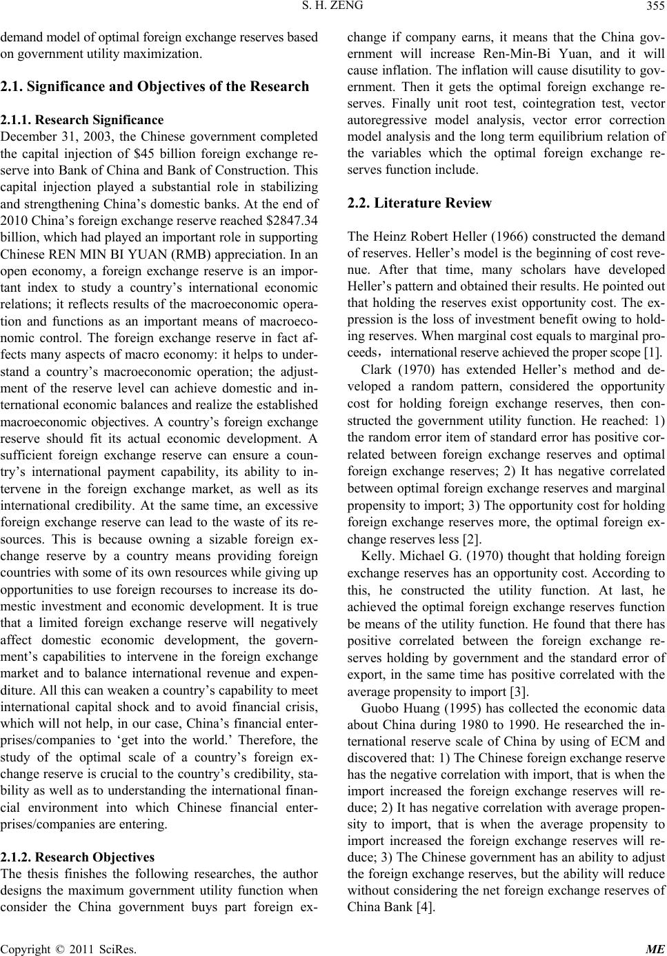 S. H. ZENG355 demand model of optimal foreign exchange reserves based on government utility maximization. 2.1. Significance and Objectives of the Research 2.1.1. Researc h Sig ni fi ca nce December 31, 2003, the Chinese government completed the capital injection of $45 billion foreign exchange re- serve into Bank of China and Bank of Construction. This capital injection played a substantial role in stabilizing and strengthening China’s domestic banks. At the end of 2010 China’s foreign exchange reserve reached $2847.34 billion, which had played an important role in supporting Chinese REN MIN BI YUAN (RMB) appreciation. In an open economy, a foreign exchange reserve is an impor- tant index to study a country’s international economic relations; it reflects results of the macroeconomic opera- tion and functions as an important means of macroeco- nomic control. The foreign exchange reserve in fact af- fects many aspects of macro economy: it helps to under- stand a country’s macroeconomic operation; the adjust- ment of the reserve level can achieve domestic and in- ternational economic balances and realize the established macroeconomic objectives. A country’s foreign exchange reserve should fit its actual economic development. A sufficient foreign exchange reserve can ensure a coun- try’s international payment capability, its ability to in- tervene in the foreign exchange market, as well as its international credibility. At the same time, an excessive foreign exchange reserve can lead to the waste of its re- sources. This is because owning a sizable foreign ex- change reserve by a country means providing foreign countries with some of its own resources while giving up opportunities to use foreign recourses to increase its do- mestic investment and economic development. It is true that a limited foreign exchange reserve will negatively affect domestic economic development, the govern- ment’s capabilities to intervene in the foreign exchange market and to balance international revenue and expen- diture. All this can weaken a country’s capability to meet international capital shock and to avoid financial crisis, which will not help, in our case, China’s financial enter- prises/companies to ‘get into the world.’ Therefore, the study of the optimal scale of a country’s foreign ex- change reserve is crucial to the country’s credibility, sta- bility as well as to understanding the international finan- cial environment into which Chinese financial enter- prises/companies are entering. 2.1.2. Research Objectives The thesis finishes the following researches, the author designs the maximum government utility function when consider the China government buys part foreign ex- change if company earns, it means that the China gov- ernment will increase Ren-Min-Bi Yuan, and it will cause inflation. The inflation will cause disutility to gov- ernment. Then it gets the optimal foreign exchange re- serves. Finally unit root test, cointegration test, vector autoregressive model analysis, vector error correction model analysis and the long term equilibrium relation of the variables which the optimal foreign exchange re- serves function include. 2.2. Literature Review The Heinz Robert Heller (1966) constructed the demand of reserves. Heller’s model is the beginning of cost reve- nue. After that time, many scholars have developed Heller’s pattern and obtained their results. He pointed out that holding the reserves exist opportunity cost. The ex- pression is the loss of investment benefit owing to hold- ing reserves. When marginal cost equals to marginal pro- ceeds,international reserve achieved the proper scope [1]. Clark (1970) has extended Heller’s method and de- veloped a random pattern, considered the opportunity cost for holding foreign exchange reserves, then con- structed the government utility function. He reached: 1) the random error item of standard error has positive cor- related between foreign exchange reserves and optimal foreign exchange reserves; 2) It has negative correlated between optimal foreign exchange reserves and marginal propensity to import; 3) The opportunity cost for holding foreign exchange reserves more, the optimal foreign ex- change reserves less [2]. Kelly. Michael G. (1970) thought that holding foreign exchange reserves has an opportunity cost. According to this, he constructed the utility function. At last, he achieved the optimal foreign exchange reserves function be means of the utility function. He found that there has positive correlated between the foreign exchange re- serves holding by government and the standard error of export, in the same time has positive correlated with the average propensity to import [3]. Guobo Huang (1995) has collected the economic data about China during 1980 to 1990. He researched the in- ternational reserve scale of China by using of ECM and discovered that: 1) The Chinese foreign exchange reserve has the negative correlation with import, that is when the import increased the foreign exchange reserves will re- duce; 2) It has negative correlation with average propen- sity to import, that is when the average propensity to import increased the foreign exchange reserves will re- duce; 3) The Chinese government has an ability to adjust the foreign exchange reserves, but the ability will reduce without considering the net foreign exchange reserves of China Bank [4]. Copyright © 2011 SciRes. ME 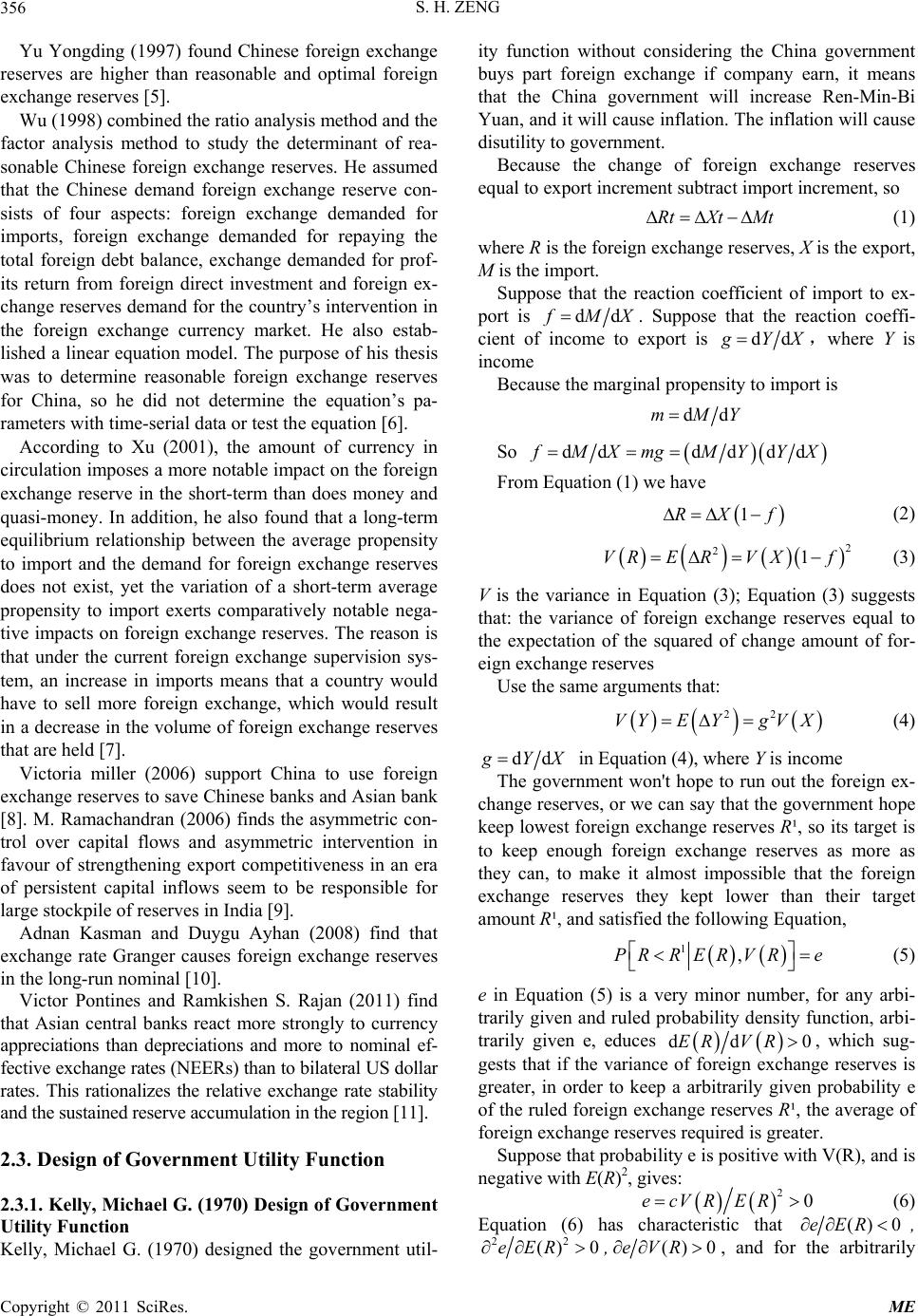 S. H. ZENG 356 Yu Yongding (1997) found Chinese foreign exchange reserves are higher than reasonable and optimal foreign exchange reserves [5]. Wu (1998) combined the ratio analysis method and the factor analysis method to study the determinant of rea- sonable Chinese foreign exchange reserves. He assumed that the Chinese demand foreign exchange reserve con- sists of four aspects: foreign exchange demanded for imports, foreign exchange demanded for repaying the total foreign debt balance, exchange demanded for prof- its return from foreign direct investment and foreign ex- change reserves demand for the country’s intervention in the foreign exchange currency market. He also estab- lished a linear equation model. The purpose of his thesis was to determine reasonable foreign exchange reserves for China, so he did not determine the equation’s pa- rameters with time-serial data or test the equation [6]. According to Xu (2001), the amount of currency in circulation imposes a more notable impact on the foreign exchange reserve in the short-term than does money and quasi-money. In addition, he also found that a long-term equilibrium relationship between the average propensity to import and the demand for foreign exchange reserves does not exist, yet the variation of a short-term average propensity to import exerts comparatively notable nega- tive impacts on foreign exchange reserves. The reason is that under the current foreign exchange supervision sys- tem, an increase in imports means that a country would have to sell more foreign exchange, which would result in a decrease in the volume of foreign exchange reserves that are held [7]. Victoria miller (2006) support China to use foreign exchange reserves to save Chinese banks and Asian bank [8]. M. Ramachandran (2006) finds the asymmetric con- trol over capital flows and asymmetric intervention in favour of strengthening export competitiveness in an era of persistent capital inflows seem to be responsible for large stockpile of reserves in India [9]. Adnan Kasman and Duygu Ayhan (2008) find that exchange rate Granger causes foreign exchange reserves in the long-run nominal [10]. Victor Pontines and Ramkishen S. Rajan (2011) find that Asian central banks react more strongly to currency appreciations than depreciations and more to nominal ef- fective exchange rates (NEERs) than to bilateral US dollar rates. This rationalizes the relative exchange rate stability and the sustained reserve accumulation in the region [11]. 2.3. Design of Government Utility Function 2.3.1. Kelly, Michael G. (1970) Design of Government Utility Function Kelly, Michael G. (1970) designed the government util- ity function without considering the China government buys part foreign exchange if company earn, it means that the China government will increase Ren-Min-Bi Yuan, and it will cause inflation. The inflation will cause disutility to government. Because the change of foreign exchange reserves equal to export increment subtract import increment, so RtXt Mt (1) where R is the foreign exchange reserves, X is the export, M is the import. Suppose that the reaction coefficient of import to ex- port is dd MX . Suppose that the reaction coeffi- cient of income to export is dd YX,where Y is income Because the marginal propensity to import is ddmMY So dddd dd MX mgMYYX From Equation (1) we have 1RX f (2) 2 21VRE RVXf (3) V is the variance in Equation (3); Equation (3) suggests that: the variance of foreign exchange reserves equal to the expectation of the squared of change amount of for- eign exchange reserves Use the same arguments that: 22 VYEYgV X (4) dd YX in Equation (4), where Y is income The government won't hope to run out the foreign ex- change reserves, or we can say that the government hope keep lowest foreign exchange reserves R¹, so its target is to keep enough foreign exchange reserves as more as they can, to make it almost impossible that the foreign exchange reserves they kept lower than their target amount R¹, and satisfied the following Equation, 1,PRRER VRe (5) e in Equation (5) is a very minor number, for any arbi- trarily given and ruled probability density function, arbi- trarily given e, educes ddER VR0 , which sug- gests that if the variance of foreign exchange reserves is greater, in order to keep a arbitrarily given probability e of the ruled foreign exchange reserves R¹, the average of foreign exchange reserves required is greater. Suppose that probability e is positive with V(R), and is negative with E(R)2, gives: 20ecVRER (6) Equation (6) has characteristic that () 0eER , 22 () 0eER ,() 0eVR , and for the arbitrarily Copyright © 2011 SciRes. ME 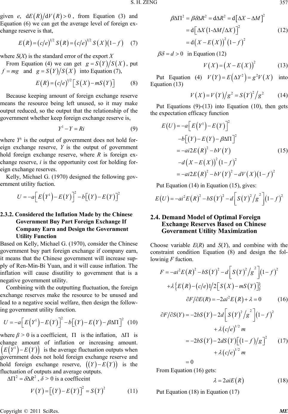 S. H. ZENG357 given e, ddER VR0, from Equation (3) and Equation (6) we can get the average level of foreign ex- change reserve is that, 1212 1ERceSRce SXf (7) where S(X) is the standard error of the export X From Equation (4) we can get SYS X, put mg and SYS X into Equation (7), 12 ERceSX mSY (8) Because keeping amount of foreign exchange reserve means the resource being left unused, so it may make output reduced, so the output that the relationship of the government whether keep foreign exchange reserve is, 1 YYRi (9) where Y¹ is the output of government does not hold for- eign exchange reserve, Y is the output of government hold foreign exchange reserve, where R is foreign ex- change reserve, i is the opportunity cost for holding for- eign exchange reserves. Kelly, Michael G. (1970) designed the following gov- ernment utility fuction. 22 1 UaEYEYbYEY 2.3.2. Considered the Inflation Made by the Chinese Government Buy Part Foreign Exchange If Company Earn and Design the Government Utility Function Based on Kelly, Michael G. (1970), consider the Chinese government buy part foreign exchange if company earn, it means that the Chinese government will increase sup- ply of Ren-Min-Bi Yuan, and it will cause inflation. The inflation will cause disutility to government that is a negative government utility. Combining with the outputting fluctuation, the foreign exchange reserves make the resource to be unused and lead to a negative social welfare, then design the follow- ing government utility function. 22 1 UaEYEYbYEY (10) where β > 0 is a coefficient, is the inflation, is change amount of inflation or increasing amount. is the average fluctuation outputs when government does not hold foreign exchange reserve and hold foreign exchange reserve, is the fluctuation of outputs and average outputs. 1 EY EY 2 YEY 2 R , δ > 0 is a coefficeint 22 VYY EYSY (11) 2 2 2 22 2 2 dd d1- d1 MX XE X Xf RR M X (12) 0d in Equation (12) 2 VXX EX (13) Put Equation (4) 22 VYEYgV X into Equation (13) 2 22 VXVY gSYg (14) Put Equations (9)-(13) into Equation (10), then gets the expectation efficacy function 2 1 2 2 22 22 2 1 21 EUa EYEY bY EY ai ERbV Y dX EXf ai ERbV YdVXf 2 (15) Put Equation (14) in Equation (15), gives: 2 22 2 21EUaiERbSYdSYgf 2 2.4. Demand Model of Optimal Foreign Exchange Reserves Based on Chinese Government Utility Maximization Choose variable E(R) and S(Y), and combine with the constraint condition Equation (8) and design the fol- lowinig F fuction. 2 22 2 21 12 2 aiERbS YdSYgf ERceSX mSY 2 () 20FER aiER (16) 2 22 1/2 2 1/2 () 221 221 0 SYbS YdSYgf ce m bS YdS Yfg ce m (17) From Equation (16) gets: 2aiE R (18) Put Equation (18) in Equation (17) Copyright © 2011 SciRes. ME  S. H. ZENG 358 2 1/2 2 22 0 1bS YdS Yfg aiRcemE (19) As a matter of convenience, arranges h as the follow- ings 1/2 hce (20) From Equation (19) and Equation (20) gets 2 21SYai ERhmbfgd (21) Put Equation (21) in Equation (8) 2 21 ER hSXmai ERhmbfgd (22) From Equation (22) gets 2 122 1 ER SXhaimhbf g d (23) Put dd MX mg in Equation (23) 2 122 1 ER SXhaimhbgm d (24) Because of 2 2 12 ER DF ai0 So 2 22 2 22 1 22210 DFER FSYFERSY aibdf g Conditions as above satisfied binary function approach maximum, that is the government expectation efficacy function E(U) exist a maximum, the optimal foreign ex- change reserves based on government utility maximiza- tion could fixed by Equation (24). Be convenient order, let 2 22 1 1khaimhb gmd (25) 2 1 wb gmd (26) 2.5. Analyze the Optimal Expectation Foreign Exchange Reserve to the Sensitivity of Variable and Parameter Based on Government Utility Maximization The foreign exchange reserve which government expec- tation utility maximization E(U) exist a maximum is the optimal expectation foreign exchange reserve E(R), to the sensitivity ER g of reaction coefficient dd YX that income to export, approach the partial derivative. 22122 2 2 ER g SXhai mdgmgkw (27) When 10gm , that is dd1fMXmg 22122 2 20 ER g SXhaim dgmgkw (28) When 10gm , that is ddfMXmg1 22122 2 20 ER g SXhaim dgmgkw (29) When 10gm , that is ddfMXmg1 22122 2 20 ER g SXhaim dgmgkw (30) So the sensitivity ERg of reaction coefficient (ddgYX ) that optimal foreign exchange reserve to reaction coefficient that import to export is depend on the size of mg , that is depend on the size of the reac- tion coefficient dd MX that import to export. The optimal foreign exchange reserve susceptibility ER m to the marginal propensity to import ddm Y, approach the partial derivative. 2222 2 2 ER m SXhaimbdgmdgkw (31) When 12 1bdmggdf g 2222 2 20 ER m SXhaimbdgmdgkw (32) When 12 1bdmggdf g 2222 2 20 ER m SXhaimbdgmdgkw (33) When 12 1bdmggdf g 2222 2 20 ER m SXhaimbdgmdgkw (34) The optimal expectation foreign exchange reserve sus- ceptibility ER SX to the export standard devia- tion S (X), approach the partial derivative, Copyright © 2011 SciRes. ME 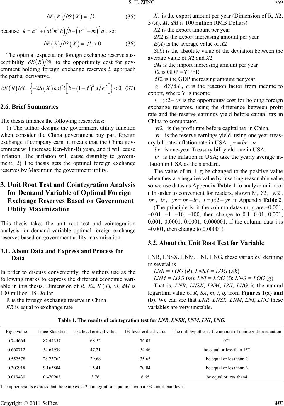 S. H. ZENG Copyright © 2011 SciRes. ME 359 1ER SXk (35) X1 is the export amount per year (Dimension of R, X2, S (X), M, dM is 100 million RMB Dollars) because 2 122 1 khaimhb gmd , so: X2 is the export amount per year dX2 is the export increasing amount per year 1ER SXk0 (36) E(X) is the average value of X2 S(X) is the absolute value of the deviation between the average value of X2 and X2 The optimal expectation foreign exchange reserve sus- ceptibility ER i to the opportunity cost for gov- ernment holding foreign exchange reserves i, approach the partial derivative, dM is the import increasing amount per year Y2 is GDP =Y1/ER 2 22 21ERiSXhai ibfdg 0 (37) dY2 is the GDP increasing amount per year dd YX , g is the reaction factor from income to export, where Y is income 2iyt yr is the opportunity cost for holding foreign exchange reserves, using the difference between profit rate and the reserve earnings yield before capital tax in China to compotator. 2.6. Brief Summaries The thesis finishes the following researches: 1) The author designs the government utility function when consider the China government buy part foreign exchange if company earn, it means that the China gov- ernment will increase Ren-Min-Bi yuan, and it will cause inflation. The inflation will cause disutility to govern- ment; 2) The thesis gets the optimal foreign exchange reserves by Maximum the government utility. 2 t is the profit rate before capital tax in China. yr is the reserve earnings yield, using one year treas- ury bill rate-inflation rate in USA rbrir br is one-year Treasury bill yield rate in USA. ir is the inflation in USA; take the yearly average in- flation in USA as the standard. The value of m, i ,g be changed to the positive value when they are negative value by inserting reasonable value, so we use datas as Appendix Table 1 to analyze unit root ( In order to convenient for readers, shown M, Y2, 2 t, , , br ir rbrir , 2iyt y 3. Unit Root Test and Cointegration Analysis for Demand Variable of Optimal Foreign Exchange Reserves Based on Government Utility Maximization r in Appendix Table 2. (The principle is, if the column datas m, g are –0.001, –0.01, –1, –10, –100, then change to 0.1, 0.01, 0.001, 0.001, 0.0001. 0.0001, 0.000001; if the column data i is –0.001, then change to 0.00001) This thesis takes the unit root test and cointegration analysis for demand variable optimal foreign exchange reserves based on government utility maximization. 3.2. About the Unit Root Test for Variable 3.1. About Data and Express and Process for Data LNR, LNSX, LNM, LNI, LNG, these variables’ defining in several is LNR = LOG (R); LNSX = LOG (SX) In order to discuss conveniently, the authors use as the following marks to express the different economic vari- able in this thesis. Dimension of R, X2, S (X), M, dM is 100 million US Dollar LNM = LOG (m); LNI = LOG (i); LNG = LOG (g) That is, LNR, LNSX, LNM, LNI, LNG is the natural logarithm value of R, SX, m, i, g, from Figures 1(a) and (b). We can see that LNR, LNSX, LNM, LNI, LNG these variables are very unstable. R is the foreign exchange reserve in China ER is equal to exchange rate Table 1. The results of cointegration test for LNR, LNSX, LNM, LNI, LNG. Eigenvalue Trace Statistics 5% level critical value1% level critical value The null hypothesis: the amount of cointegration equation 0.744664 87.44357 68.52 76.07 0** 0.660712 54.67939 47.21 54.46 be equal or less than 1** 0.557578 28.73762 29.68 35.65 be equal or less than 2 0.303918 9.165804 15.41 20.04 be equal or less than 3 0.019430 0.470908 3.76 6.65 be equal or less than4 The upper results express that there are exist 2 cointegration equations with a 5% significant level. 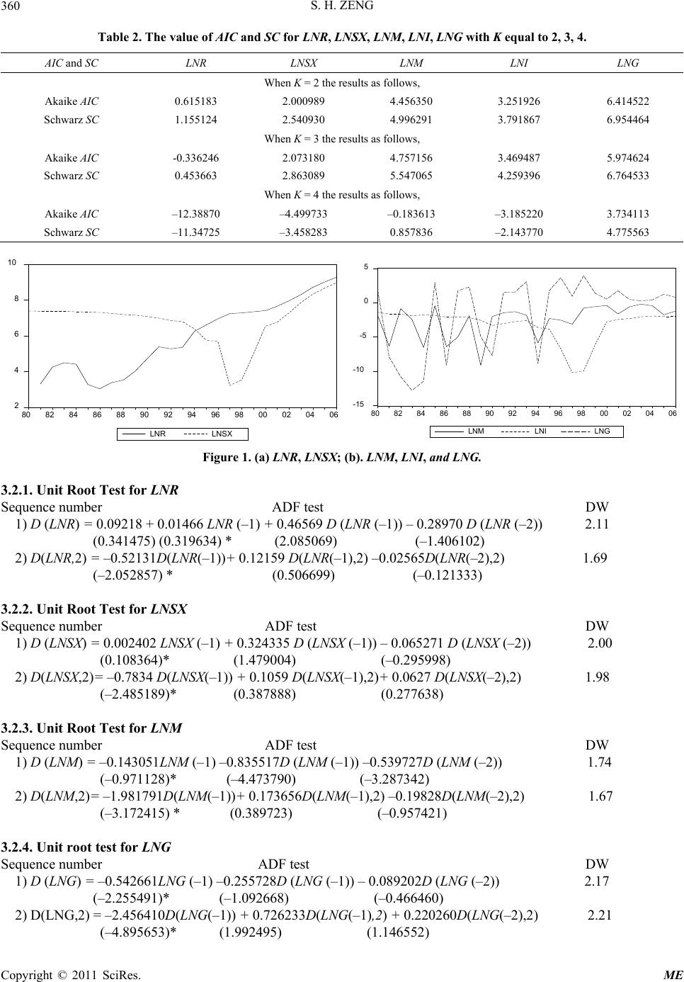 S. H. ZENG 360 Table 2. The value of AIC and SC for LNR, LNSX, LNM, LNI, LNG with K equal to 2, 3, 4. AIC and SC LNR LNSX LNM LNI LNG When K = 2 the results as follows, Akaike AIC 0.615183 2.000989 4.456350 3.251926 6.414522 Schwarz SC 1.155124 2.540930 4.996291 3.791867 6.954464 When K = 3 the results as follows, Akaike AIC -0.336246 2.073180 4.757156 3.469487 5.974624 Schwarz SC 0.453663 2.863089 5.547065 4.259396 6.764533 When K = 4 the results as follows, Akaike AIC –12.38870 –4.499733 –0.183613 –3.185220 3.734113 Schwarz SC –11.34725 –3.458283 0.857836 –2.143770 4.775563 2 4 6 8 10 80 82 84 86 88 90 92 94 96 98 00 020406 LNR LNSX -15 -10 -5 0 5 80 82 84 86 88 90 92 94 96 98 00 02 04 06 LNMLNILNG Figure 1. (a) LNR, LNSX; (b). LNM, LNI, and LNG. 3.2.1. Unit Root Test for LNR Sequence number ADF test DW 1) D (LNR) = 0.09218 + 0.01466 LNR (–1) + 0.46569 D (LNR (–1)) – 0.28970 D (LNR (–2)) 2.11 (0.341475) (0.319634) * (2.085069) (–1.406102) 2) D(LNR,2) = –0.52131D(LNR(–1))+ 0.12159 D(LNR(–1) ,2) –0 .02565D(LNR(–2),2) 1.69 (–2.052857) * (0.506699) (–0.121333) 3.2.2. Unit Root Test for LNSX Sequence number ADF test DW 1) D (LNSX) = 0.002402 LNSX (–1) + 0.3243 35 D (LNSX (–1)) – 0.065271 D (LNSX (–2)) 2.00 (0.108364)* (1.479004) (–0.295998) 2) D(LNSX,2)= –0.7834 D(LNSX(–1 )) + 0.1059 D(LNSX(–1),2)+ 0.0627 D(LNSX(–2),2) 1.98 (–2.485189)* (0.387888) (0.277638) 3.2.3. Unit Root Test for LNM Sequence number ADF test DW 1) D (LNM) = –0.143051LNM (–1) –0.835517D (LNM (–1)) –0.539727D (LNM (–2)) 1.74 (–0.971128)* (–4.473790) (–3.287342) 2) D(LNM,2)= –1.981791D(LNM(–1))+ 0.173656D(LNM(–1),2) –0.19828D(LNM(–2),2) 1.67 (–3.172415) * (0.389723) (–0.957421) 3.2.4. Unit root test for LNG Sequence number ADF test DW 1) D (LNG) = –0.542661LNG (–1) –0.25572 8D (LNG (–1)) – 0.089202D (LNG (–2)) 2.17 (–2.255491)* (–1.092668) (–0.466460) 2) D(LNG,2) = –2.456410D(LNG(– 1)) + 0.72 6233D(LNG(–1),2 ) + 0.220260D(LNG(–2),2) 2.21 (–4.895653)* (1.992495) (1.146552) Copyright © 2011 SciRes. ME 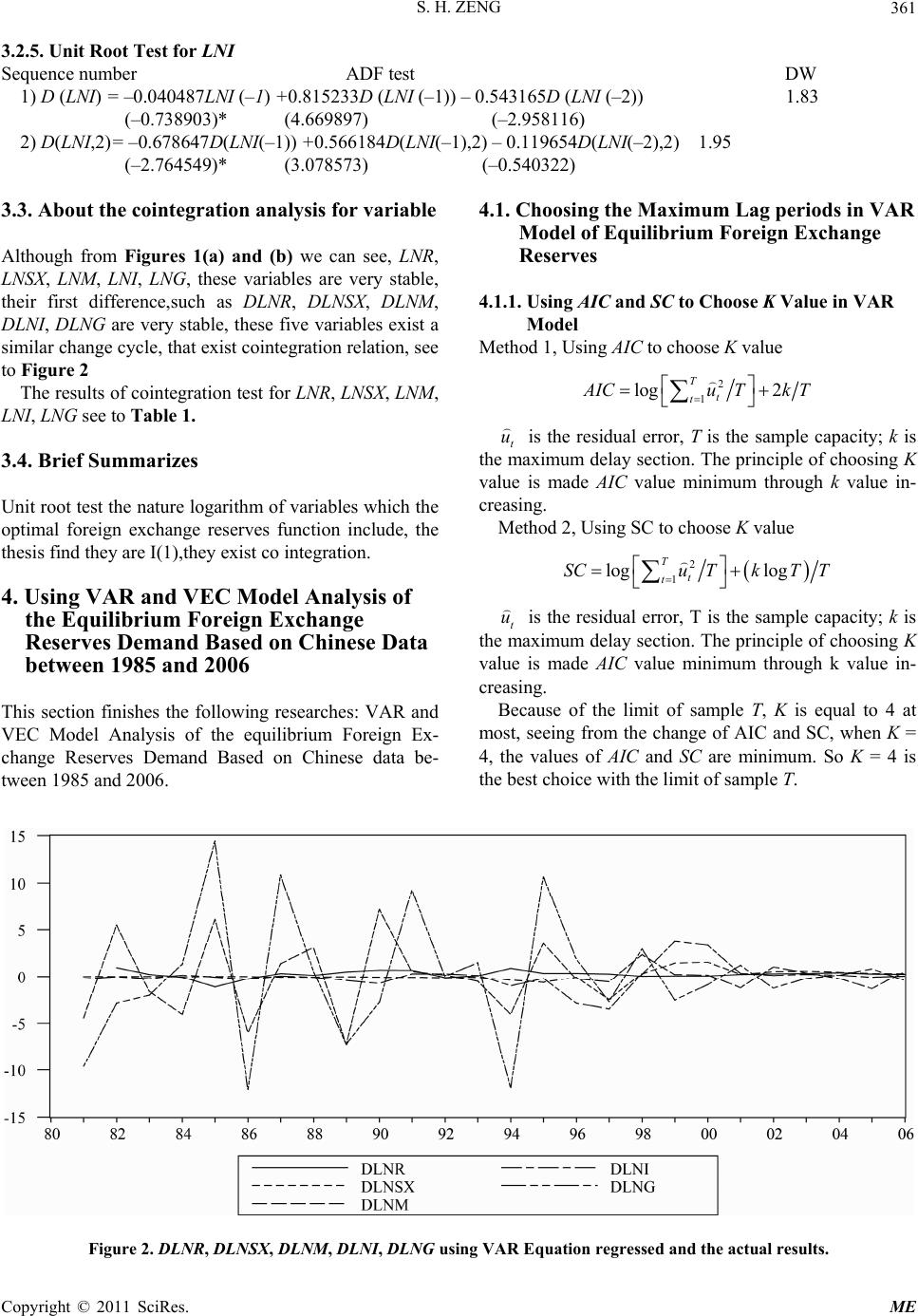 S. H. ZENG Copyright © 2011 SciRes. ME 361 3.2.5. Unit Root Test for LNI Sequence number ADF test DW 1) D (LNI) = –0.040487 LNI (–1) +0.815233D (LNI (–1)) – 0.543165D (LNI (–2)) 1.83 (–0.738903)* (4.669897) (–2.958116) 2) D(LNI,2)= –0.678647D(LNI(–1)) +0.566184D(LNI(–1),2) – 0.119654D(LNI(–2),2) 1.95 (–2.764549)* (3.078573) (–0.540322) 3.3. About the cointegration analysis for variable 4.1. Choosing the Maximum Lag periods in VAR Model of Equilibrium Foreign Exchange Reserves Although from Figures 1(a) and (b) we can see, LNR, LNSX, LNM, LNI, LNG, these variables are very stable, their first difference,such as DLNR, DLNSX, DLNM, DLNI, DLNG are very stable, these five variables exist a similar change cycle, that exist cointegration relation, see to Figure 2 4.1.1. Using AIC and SC to Choose K Value in VAR Model Method 1, Using AIC to choose K value 2 1 log 2 T t t ICuTkT The results of cointegration test for LNR, LNSX, LNM, LNI, LNG see to Tab le 1. t u is the residual error, T is the sample capacity; k is the maximum delay section. The principle of choosing K value is made AIC value minimum through k value in- creasing. 3.4. Brief Summarizes Unit root test the nature logarithm of variables which the optimal foreign exchange reserves function include, the thesis find they are I(1),they exist co integration. Method 2, Using SC to choose K value 2 1 log log T t t SCu TkT T 4. Using VAR and VEC Model Analysis of the Equilibrium Foreign Exchange Reserves Demand Based on Chinese Data between 1985 and 2006 t u is the residual error, T is the sample capacity; k is the maximum delay section. The principle of choosing K value is made AIC value minimum through k value in- creasing. Because of the limit of sample T, K is equal to 4 at most, seeing from the change of AIC and SC, when K = 4, the values of AIC and SC are minimum. So K = 4 is the best choice with the limit of sample T. This section finishes the following researches: VAR and VEC Model Analysis of the equilibrium Foreign Ex- change Reserves Demand Based on Chinese data be- tween 1985 and 2006. Figure 2. DLNR, DLNSX, DLNM, DLNI, DLNG using VAR Equation regressed and the actual results.  S. H. ZENG Copyright © 2011 SciRes. ME 362 4.1.2. VAR Model of Equilibrium Foreign Exchange Reserves Demand Based on C h in e se Data Between 1985 and 2006 Because K = 4 is the best choice, VAR model of equilib- rium foreign exchange reserves demand based on Chi- nese data between 1985 and 2006 used K = 4, when the variable delayed 4 sections, that is when K = 4 the Equtions as follows, LNR = 1.158208*LNR(–1) – 0.75956090 28* LNR(–2) + 1.275854675*LNR(–3) – 0.41874649*LNR(–4) – 0.5326487006*LNSX(–1) + 0.04889939 537*LNSX(–2) + 0.272843226*LNSX(–3) – 0.039302859*LNSX(–4) – 0.01712404005*LNM(–1) – 0.1990991828*LNM(–2) – 0.1133346012*LNM(–3) – 0.03947680 86*LNM(–4) + 0.3329742763*LNI(–1) + 0.1276036813*LNI(–2) – 0.1739915379*LNI(–3) + 0.0949172971*LNI(–4) + 0.0309059384*LNG(–1) + 0.071224 90 394*LNG(–2) + 0.05650023494*LNG(–3) + 0.01177553 108 *LNG(–4) + 1.07792509 LNSX = –3.938060 6*LNR(–1) + 3.35668*LNR(–2) – 0.607910938*LNR(–3) + 0.5289359612*LNR(–4) + 1.752410011*LNSX(–1) + 0.7814465787*LNSX(–2) – 0.96916476*LNSX(–3) + 0.3469152308*LNSX (–4) + 0.02346185581*LNM(–1) + 0.380843381*LNM(–2 ) + 0.02583196853*LNM(–3) – 0.1368834866*LNM(–4) – 0.2797186513*LNI(–1) – 1.013477322*LNI(–2) + 1.247770225*LNI(–3) – 0.455388757*LNI(–4) – 0.05458893085* LNG(–1) – 0.0383 9642266*LNG(–2) + 0.1945562552*LNG(–3) + 0.2417625189*LNG(–4) – 1.52559448 LNI = – 8.618872*LNR(–1) + 9.4407164*LNR(–2) – 6.7190925*LNR(–3) + 3.102998318*LNR(–4) + 5.061829074*LNSX(–1) – 1.173982425*LNSX(–2) – 1.455715567*LNSX(–3) + 2.734477293*LNSX(–4) + 0.6480708563*LNM(–1) + 1.557535337*LNM(–2) + 0.2412607597*LNM(–3) – 0.09576680591*LNM(–4) – 2.139039105*LNI(–1) – 0.418124 08 94*LNI(–2) + 2.005046131*LNI(–3) – 1.968406804*LNI(–4) – 0.342939926*LNG(–1) – 0.1883294592*LNG(–2) + 0.4212904271*LNG(–3) + 0.355278824*LNG(–4) – 21.58283256 LNG = 14.175261*LNR(–1) – 18.4748659*LNR(–2) + 8.1032935*LNR (– 3) + 3.35 161008 *LNR(–4) – 10.54483977*LNSX(–1) + 2.4 11978668*LNSX(–2) + 5.86210599*LNSX(–3) – 2.55802 967*LNSX(–4) – 0.0052018235*LNM(–1) – 1.774668358*LNM( –2) – 1.075279662*LNM(–3) – 1.741231895*LNM(–4) + 5.55427464*LNI(–1) – 0.99946 07549*LNI(–2) – 2.685201432*LNI(–3) + 1.629023047*LNI(–4) – 0.157488914*LNG(–1) – 0.1861 27449*LNG(–2) – 0.8664866224*LNG(–3) + 0.02690099581*LNG(–4) – 10.87342161 Using LNR equation in VAR equation set to forecast the foreign exchange reserve in China (FR), the fore- casting values of FR and the actual values of R are shown in Figure 3 and Table 3. See from Table 3 the forecast error is very minor, from 0.02% to 0.1%, and the forecasting is highly accurate, from 99.98% to 99.99%. 4.2. VEC Model Estimation of Equilibrium Foreign Exchange Reserves Demand Based on Chinese Data Between 1985 and 2006 Because all the values LNR, LNSX, LNM, LNI, LNG are I(1), also exist co integration, so exist a error correction model. 4.2.1. Det e rm i n in g t h e Delay Section in the VEC Model of the Equilibrium Foreign Exchange Reserves Demand Based on t he C h in es e Data between 1985 and 2006 Because when K = 1 Akaike Information Criteria 15.69124 Schwarz Criteria 17.65466 When K = 2 Akaike Information Criteria 13.59685 Schwarz Criteria 16.80585 Figure 3. The forecasting values of FR and the actual values of R.  S. H. ZENG363 Table 3. Forecast error between the value of FR and R. obs RESID R FR ES 1985 0.01 26.44 26.435 0.0002 1986 0.01 20.72 20.709 0.0006 1987 0.01 29.23 29.222 0.0003 1988 0.01 33.72 33.71 0.0003 1989 0.02 55.5 55.485 0.0003 1990 0.07 110.93 110.86 0.0006 1991 0.11 217.12 217.01 0.0005 1992 0.12 194.43 194.31 0.0006 1993 0.11 211.99 211.88 0.0005 1994 0.31 516.2 515.89 0.0006 1995 0.64 735.97 735.33 0.0009 1996 0.72 1050.3 1049.6 0.0007 1997 1.02 1398.9 1397.9 0.0007 1998 1.09 1449.6 1448.5 0.0008 1999 1.11 1546.8 1545.7 0.0007 2000 1.39 1655.7 1654.3 0.0008 2001 1.62 2121.7 2120.1 0.0008 2002 2.16 2864.1 2861.9 0.0008 2003 4.09 4032.5 4028.4 0.001 2004 2.81 6099.3 6096.5 0.0005 2005 12.3 8188.7 8176.4 0.0015 2006 7.54 10663 10656 0.0007 2007 22283 So K = 2 is the best choice of cointegration equation and error correction model with the limit of sample ca- pacity, gets the VEC model as follows, 4.2.2. VEC Model Estimation Results of Equilibrium Foreign Exchange Re serves Demand Based on Chinese data between 1985 and 2006 4.2.2.1. Delay section K = 1 D(LNR) = –0.02082643444*( LNR(–1) – 0.81557953*LNSX(–1) – 0.91636494*LNM(–1) + 0.71058393*LNI(–1) – 0.04742 8193*LNG(–1) – 0.3588416363 ) + 0.25008865*D(LNR(–1)) + 0.1427340478*D (LNSX(–1)) + 0.02230181302*D(LNM(–1)) – 0.06450460302*D (LNI(–1)) – 0.02126208418*D(LNG(–1)) + 0.1450919242 D(LNSX) = 0.03164245422*( LNR(–1) – 0.815579531*LNSX(–1) – 0.9163649488*LNM( –1) + 0.710583936*LNI(–1) – 0.0474281939*LNG(–1) – 0.358841636 ) – 0.20362 37*D(LNR(–1)) – 0.64870222*D(LNSX(–1)) + 0.0517247267*D (LNM(–1)) + 0.5572220392*D(LNI(–1)) – 0.02544716867*D(LNG(–1)) + 0.15891 21152 D(LNM) = 1.220107884*( LNR(–1) – 0.8155795318*LNSX(–1) – 0.9163649488*LNM(–1) + 0.710583936*LNI(–1) – 0.0474281939* LNG(–1) – 0.358841636) + 0. 888630 89*D(LNR(–1)) – 0.9519198157*D(LNSX(– 1)) – 0.008114850993*D(LNM(–1)) + 0.2931732124*D (LNI(–1)) + 0.04427418309*D(LNG(–1)) – 0.1860917443 D(LNI) = –0.3332935656*( LNR(–1) – 0.81557953*LNSX(–1) – 0.9163649488*LNM(–1) + 0.710583936*LNI(–1) – 0.047428193*LNG(–1) – 0.358841636 ) + 0.0313 8545*D (LNR(–1)) – 0.6885940951*D (LNSX(–1)) Copyright © 2011 SciRes. ME  S. H. ZENG 364 – 0.07677391686*D (LNM(–1)) + 0.7975711815*D (LNI(–1)) – 0.08023819174*D (LNG(–1)) + 0.07411662228 D(LNG) = 2.164457793*( LNR(–1) – 0.8155795318*LNSX(–1) – 0.9163649488*LNM(–1) + 0.710583936*LNI(–1) – 0.0474281939*LNG(–1) – 0.35884163 ) – 0.64807905*D(LNR(–1)) – 2.3799935*D(LNSX(–1)) + 0.7679206802*D(LNM(–1)) + 0.8411639391*D (LNI(–1)) – 0.3874419347*D (LNG(–1)) + 0.7787188403 The long term equilibrium relation of these variables LNR, LNSX, LNM, LNI, LN are, LNR (–1) = 0.8155 795318*LNSX (–1) + 0.9163649488*LNM (–1) – 0.7105839363*LNI (–1) + 0.04742819394*LNG (–1) + 0.3588416 363 4.2.2.2. Delay Section K = 2 D(LNR) = 0.0210919311*( LNR (–1) – 8.39646148*LNSX(–1) – 6.53172328* LNM(–1) + 9.319611202*LNI(–1) + 5.92161891 5*LNG(–1) + 72.52744886 ) – 0.4199163 335*D (LNR(–1)) + 0.02744055717*D(LNR(–2)) + 0.178363838*D (LNSX(–1)) – 0.07798941*D(LNSX(–2)) + 0.1637*D(LNM(–1)) + 0.100098*D(LNM(–2)) – 0.210331*D(LNI(–1)) + 0.043212*D(LNI(–2)) – 0.13208757*D(LNG(–1)) – 0.07503047391*D (LNG(–2)) + 0.3559304786 D(LNSX) = 0.0099460 85465*( LNR(–1 ) – 8.396461487*LNSX(–1) – 6.531723289*LNM(–1) + 9.3196112*LNI(– 1) + 5.92161891 5*LNG(–1) + 72.52744886 ) – 0.9757317399*D (LNR(–1)) + 0.2452650037*D (LNR(–2)) + 0.0633299*D(LNSX(–1)) + 0.622115*D(LNSX(–2)) + 0.063976*D(LNM(–1)) + 0.03197 *D(LNM(–2)) + 0.34938*D(LNI(–1)) – 0.55305 4*D(LNI(–2)) – 0.09832038718*D(LNG(–1)) – 0.0638524772*D (LNG(–2)) + 0.25181 44464 D(LNM) = –0.028990184*( LNR (–1) – 8.396461487*LNSX(–1) – 6.531723289*LNM(–1) + 9.319611202*LNI(–1) + 5.921618915*LNG(–1) + 72.52744886 ) + 3.9950447*D(LNR(–1)) – 0.9449371943*D (LNR(–2)) + 0.23898574*D(LNSX(–1)) + 0.55443735*D (LNSX(–2)) – 1.12316*D(LNM(–1)) – 0.6771437*D(LNM(–2) ) + 0.3818*D(LNI(–1)) – 0.830993*D(LNI(–2)) + 0.2355717803*D (LNG(–1)) + 0.09248289596*D(LNG(–2)) – 0.6183 532604 D(LNI) = – 0.01178074236*( LNR(– 1) – 8.3964614*LNSX (–1) – 6.53172 3289*LNM(–1) + 9.319611202*LNI(–1) + 5.92161891*LNG(–1) + 72.5274488 ) – 0.1287365454*D(LNR(–1)) – 0.5332005646*D(LNR(–2 )) – 0.04472733462*D (LNSX(–1)) + 0.3249581422*D(LNSX(–2)) + 0.0638542*D(LNM(–1) ) + 0.0026686*D(LNM(–2)) + 0.852404135*D(LNI(–1)) – 0.72172054*D(LNI(–2)) – 0.052984839*D(LNG(–1)) + 0.002247385*D (LNG(–2)) + 0.1702761775 D(LNG) = –0.3047102393*( LNR(–1) – 8.396461487*LNSX(–1) – 6.53172 3289*LNM(–1) + 9.319611202*LNI(–1) + 5.92161891 5*LNG (–1) + 72.52744886) + 14.95319432*D(LNR(–1)) – 4.995081418*D(LNR(–2)) – 3.7942098*D(LNSX(–1)) + 0.42273224*D(LNSX(–2)) – 1.7528*D(LNM(–1)) – 1.626889*D(LNM(–2)) + 2.911406* D(LNI(–1)) + 0.211057*D(LNI(–2)) + 1.112724587*D(LNG(–1)) + 0.8964220686*D(LNG(–2)) – 1.644163043 So the long term equilibrium relation of these vari- ables LNR(–1), LNSX(–1), LNM(–1), LNI(–1), LNG(–1) are LNR(–1) = 8.39646148 7*LNSX(–1) + 6.531723289*LNM(–1) – 9.319611202*LNI(–1) – 5.921618915*LNG(–1) – 72.52744886 The upper equation express that, the elasticity that the Chinese foreign exchange reserves to export standard deviation (SX) is 8.396461487, it means that the export standard deviation increased 1%, the foreign exchange reserves will increase 8.396461487%.The elasticity that the Chinese foreign exchange reserves to the marginal propensity to import (m) is 6.531723289, it means that the marginal propensity to import increased 1%, the for- eign exchange reserves will increase 6.531723289%.It can be explained that, the marginal propensity to import means the unit output increased will caused more import, so more reserves are necessary for the need of import. The elasticity of the Chinese foreign exchange re- serves to the net opportunity cost (i)1 is –9.319611202, it means that the net opportunity cost of hold foreign ex- change reserves increased 1%; the Chinese foreign ex- change reserves will reduce 9.319611202%. The elasticity between the foreign exchange reserves and the reaction coefficient of income to export is – 5.921618915, it means that the reaction coefficient of income to export increased 1%, the foreign exchange reserves will reduce 5.921618915. It can be explained that, the reaction coefficient of in- come to export is g increased, means that the increased unit export will lead to the unit output increase, and then increased the export lead to the foreign exchange re- 1net opportunity cost = return rate of capital – return rate of Chinese foreign exchange reserves. Copyright © 2011 SciRes. ME  S. H. ZENG Copyright © 2011 SciRes. ME 365 serves increase, so the government should cut the hold- ing foreign exchange reserves to make the government utility maximization. 3.2.2.3. Compared the Forecasting the Foreign Exchange Reserves with the Actual Foreign Exchange Reserves in the Long Term Equilibrium Relation with Delay Section K = 1 and K = 2 Suppose that FLLNR is the forecast of LNR in the long term equilibrium relation with delay section K = 1, gives the equation, FLLNR = 0.815579531 8*LNSX (–1) + 0.9163649488*LNM (–1) – 0.7105 839363 *LNI (–1) + 0.04742819394* LNG (–1 ) + 0.3588 41636 3 FLR is the forecast of R in long term equilibrium rela- tion, gives the equation, FLR = 2.718^ FLLNR Suppose FLLNR2 is the forecast of LNR in long term equilibrium relation with delay section K = 2, gives the equation, FLLNR2 = 8.396461487*LNSX(–1) + 6.531723289*LNM(–1) – 9.319611202*LNI(–1) – 5.921618915*LNG(–1) – 72.52744886 FLR2 is the forecast of LNR in long term equilibrium relation with delay section K = 2, gives the equation, FLR2 = 2.718^ FLLNR The results of forecasts are shown in Table 4 and Figure 4. Table 4. The values comparing between the forecasting foreign exchange reserves and Actual foreign exchange reserves in long term equilibrium relation with delay section K = 1 and K = 2. ar R FLR FLR2 RESID DR R/FLR 1981 27.08 304.1448779 304.1448779 –277.1 –0.911 0.089 1982 69.89 3.929199758 3.929199758 65.961 16.787 17.787 1983 89.01 520.8666099 520.8666099 –431.9 –0.829 0.1709 1984 82.2 127.0019411 127.0019411 –44.8 –0.353 0.6472 1985 26.44 2.931360374 2.931360374 23.509 8.0197 9.0197 1986 20.72 1598.467981 1598.467981 –1578 –0.987 0.013 1987 29.23 4.615698492 4.615698492 24.614 5.3327 6.3327 1988 33.72 25.47169536 25.47169536 8.2483 0.3238 1.3238 1989 55.5 455.7770815 455.7770815 –400.3 –0.878 0.1218 1990 110.93 0.557141842 0.557141842 110.37 198.11 199.11 1991 217.12 539.6117699 539.6117699 –322.5 –0.598 0.4024 1992 194.43 1037.334284 1037.334284 –842.9 –0.813 0.1874 1993 211.99 886.7690989 886.7690989 –674.8 –0.761 0.2391 1994 516.2 507.0328202 507.0328202 9.1672 0.0181 1.0181 1995 735.97 10.75360771 10.75360771 725.22 67.439 68.439 1996 1050.29 320.0219763 320.0219763 730.27 2.2819 3.2819 1997 1398.9 1991.527008 1991.527008 –592.6 –0.298 0.7024 1998 1449.6 1641.464691 1641.464691 –191.9 –0.117 0.8831 1999 1546.8 17435.01253 17435.01253 –15888 –0.911 0.0887 2000 1655.7 4232.041229 4232.041229 –2576 –0.609 0.3912 2001 2121.7 1524.305782 1524.305782 597.39 0.3919 1.3919 2002 2864.1 487.0255929 487.0255929 2377.1 4.8808 5.8808 2003 4032.5 1658.261504 1658.261504 2374.2 1.4318 2.4318 2004 6099.3 3153.68506 3153.68506 2945.6 0.934 1.934 2005 8188.7 3401.096381 3401.096381 4787.6 1.4077 2.4077 2006 10663.4 1489.350917 1489.350917 9174 6.1598 7.1598  S. H. ZENG 366 Figure 4. The values comparing between the forecasting foreign exchange reserves and Actual foreign exchange reserves in long term equilibrium relation with delay section K = 1 and K = 2. I analyzed the Table 4. to find that: 1) The values of forecasting foreign exchange reserves in long term equi- librium relation with either delay section K = 1 or K = 2 are the same; 2) The ratio R/FLR is equal to 1 express that the values of actual foreign exchange reserve and long-term equilibrium are the same. If it less than 1, it express that the actual value is less than the long-term equilibrium. If it more than 1, it express that the actual value is bigger than the long-term equilibrium; 3) From Table 4 we can find that the actual foreign exchange re- serves bigger than the long-term equilibrium in 1982, 1985, 1987, 1990, 1995, 2002, 2006, and it is steady ba- sically in 1994. The value of actual foreign exchange reserves is much bigger than the long-term equilibrium in these years 1982, 1990, 1995. Because the actual value is much bigger than the long-term equilibrium in 1990, The situation supply basis for Ren-Min-Bi ex- change rate reform of China in 1994, Ren-Min-Bi ex- change rate select one kind of exchange rate and super- visory floating exchange rate institution.Because the ac- tual value is much bigger than the long-term equilibrium in 1995, the situation supply basis for Ren-Min-Bi free exchange under current account in 1996; 4)From Figure 4 we can see that the Chinese actual foreign exchange reserves are bigger than the long-term equilibrium for- eign exchange reserves in 1982, 1985, 1987, 1990, 1995, 2002, 2006.The Chinese actual foreign exchange re- serves are bigger than the long-term equilibrium foreign exchange reserves in 1982, 1990, 1995. They are nearly equal in 1994. The Chinese actual foreign exchange re- serves are smaller than the long-term equilibrium foreign exchange reserves in 1981, 1986, 1999. The Chinese actual foreign exchange reserves are smaller than the long-term equilibrium foreign exchange reserves in 1999 for weak world economy. This section chooses the VAR Regress finds the fitted value and actual value of foreign exchange reserves is nearly equal within 99.8%. Finally it gets the long term equilibrium relation of the nature logarithm of variables by VEC model, which are foreign exchange reserves, standard error of export, marginal propensity to import, the opportunity cost for foreign exchange reserves, mar- ginal output to export. 5. Summarizes for This thesis The thesis finishes the following researches: 1) The author designs the government utility function when consider the China government buy part foreign exchange if company earn, it means that the China gov- ernment will increase Ren-Min-Bi yuan, and it will cause inflation. The inflation will cause disutility to govern- ment. 2) The thesis gets the optimal foreign exchange re- serves by Maximum the government utility. 3) Unit root test the nature logarithm of variables which the optimal foreign exchange reserves function include, the thesis find they are I(1),they exist co integra- tion. 4) VAR Regress finds the fitted value and actual value of foreign exchange reserves is nearly equal within 99.8%. 5) The thesis gets the long term equilibrium relation of the nature logarithm of variables by VEC model, which are foreign exchange reserves, standard error of export, marginal propensity to import, the opportunity cost for foreign exchange reserves, marginal output to export. 6) The Chinese actual foreign exchange reserves are bigger than the long-term equilibrium foreign exchange reserves in 1982,1985,1987,1990,1995,2002,2006.The Chinese actual foreign exchange reserves are more big- ger than the long-term equilibrium foreign exchange re- serves in 1982, 1990, 1995.They are nearly equal in 1994. The Chinese actual foreign exchange reserves are smaller than the long-term equilibrium foreign exchange reserves in 1981, 1986, 1999. The Chinese actual foreign ex- change reserves are smaller than the long-term equilib- Copyright © 2011 SciRes. ME  S. H. ZENG367 rium foreign exchange reserves in 1999 for weak world economy. Different from the Kelly, Michael G. (1970) [3], Kelly, Michael G. (1970) designed the government utility func- tion without considering the China government buy part foreign exchange if company earn, it means that the China government will increase Ren-Min-Bi yuan, and it will cause inflation. The inflation will cause disutility to government. Finally it gets the optimal fuction, we can find through the sample data about 46 countries from 1953 to 1965, (1) the government-holding foreign ex- change reserves has positive correlation with the export standard error, (2) it has positive correlation with the average propensity to import [3]. This thesis designed the government utility function when consider the China government buy part foreign exchange if company earn, it means that the China gov- ernment will increase Ren-Min-Bi yuan, and it will cause inflation. The inflation will cause disutility to govern- ment. Finally it gets the optimal fuction, using the sam- ple datas in China 1980-2006 and VEC we can find: 1) The government-holding foreign exchange reserves has positive correlation with the export standard error; 2) It has positive correlation with the marginal propensity to import. The optimal fuction, data and regression method are all different, but all have the positive correlation be- tween the foreign exchange reserves and export standard error, also is consonant with the results about the mar- ginal propensity to import basically. Different from Guobo Huang (1995), Guobo Huang (1995) collected the correlative economic datas from 1980 to 1990 in China, using ECM based on the quar- terly datas to research the international reserves scale and discovered that: 1) The Chinese foreign exchange reserve has the negative correlation with import, that is when the import increased the foreign exchange reserves will re- duce; 2) it has negative correlation with average propen- sity to import, that is when the average propensity to import increased the foreign exchange reserves will re- duce. The thesis find that the elasticity that the Chinese foreign exchange reserves to the marginal propensity to import (m) is 6.531723289, it means that the marginal propensity to import increased 1%, the foreign exchange reserves will increase 6.531723289%.It can be explained that, the marginal propensity to import means the unit output increased will caused more import, so more re- serves are necessary for the need of import. 6. Acknowledgements I would like to thank reviewer for their opinions, and thank proffessor Yuding Yu. 7. References [1] H. R. Heller, “Optimal International Reserves,” The Economic Journal, Vol. 76, No. 302, 1966, pp. 296-308. [2] P. B. Clark, “Optimum International Reserves and the Speed of Adjustment,” Journal of Political Economy, Vol. 78, No. 2, pp. 356-376. [3] M. G. Kelly, “The Demand for International Reserves,” American Economic Review, Vol. 60, No. 4, pp. 655-667. [4] G. B. Huang, “Modeling China’s Demand for Interna- tional Reserves,” Applied Financial Economics, Vol. 5, No. 5, pp. 357-366. doi:10.1080/758522763 [5] Y. D. Yu, “Some Problems on Foreign Exchange Re- serves and International Balances,” World Economics and Polics, No. 10, 1997, pp.18-23. [6] J. Wu, “The Analysis and Affirmation of the China For- eign Exchange Reserves,” Economy Research Journal, Vol. 33, No. 6, 1998, pp. 20-29. [7] C. M. Xu, “The Reality of the Demand of the Foreign Exchange Reserves in China,” Quantitative and Techni- cal Economics, 2001, No. 12, pp. 101-103. [8] M. Victoria, “Getting out from between a Rock and a Hard Place: Can China Use Its Foreign Exchange Re- serves to Save Its Banks?” Journal of International Fi- nancial Markets, Institutions and Money, Vol. 16, No. 4, 2006, pp. 345-354. [9] M. Ramachandran, “On the Upsurge of Foreign Ex- change Reserves in India,” Journal of Policy Modeling, Vol. 28, No. 7, 2006, pp. 797-809. doi:10.1016/j.jpolmod.2006.04.006 [10] K. Adnan and D. Ayhan, “Foreign Exchange Reserves and Exchange Rates in Turkey: Structural Breaks, Unit Roots and Cointegration,” Economic Modelling, Vol. 25, No. 1, 2008, pp. 83-92. [11] V. Pontines and R. S. Rajan, “Foreign Exchange Market Intervention and Reserve Accumulation in Emerging Asia: Is there Evidence of Fear of Appreciation?” Eco- nomics Letters, Vol. 111, No. 3, 2011, pp. 252- 255. doi:10.1016/j.econmod.2007.04.010 Copyright © 2011 SciRes. ME 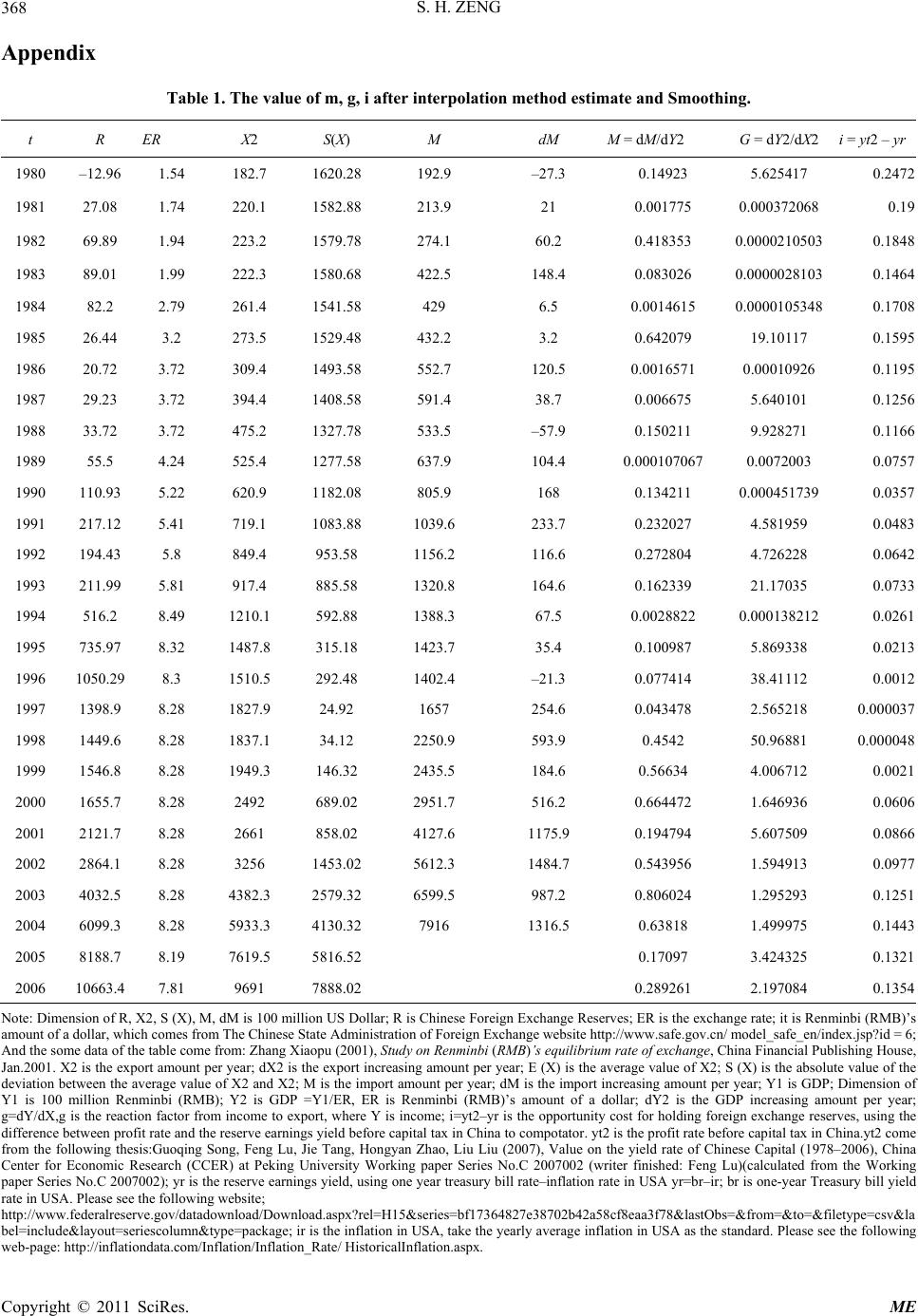 S. H. ZENG 368 Appendix Table 1. The value of m, g, i after interpolation method estimate and Smoothing. t R ER X2 S(X) M dM M = dM/dY2 G = dY2/dX2 i = yt2 – yr 1980 –12.96 1.54 182.7 1620.28 192.9 –27.3 0.14923 5.625417 0.2472 1981 27.08 1.74 220.1 1582.88 213.9 21 0.001775 0.000372068 0.19 1982 69.89 1.94 223.2 1579.78 274.1 60.2 0.418353 0.0000210503 0.1848 1983 89.01 1.99 222.3 1580.68 422.5 148.4 0.083026 0.0000028103 0.1464 1984 82.2 2.79 261.4 1541.58 429 6.5 0.0014615 0.0000105348 0.1708 1985 26.44 3.2 273.5 1529.48 432.2 3.2 0.642079 19.10117 0.1595 1986 20.72 3.72 309.4 1493.58 552.7 120.5 0.0016571 0.00010926 0.1195 1987 29.23 3.72 394.4 1408.58 591.4 38.7 0.006675 5.640101 0.1256 1988 33.72 3.72 475.2 1327.78 533.5 –57.9 0.150211 9.928271 0.1166 1989 55.5 4.24 525.4 1277.58 637.9 104.4 0.000107067 0.0072003 0.0757 1990 110.93 5.22 620.9 1182.08 805.9 168 0.134211 0.000451739 0.0357 1991 217.12 5.41 719.1 1083.88 1039.6 233.7 0.232027 4.581959 0.0483 1992 194.43 5.8 849.4 953.58 1156.2 116.6 0.272804 4.726228 0.0642 1993 211.99 5.81 917.4 885.58 1320.8 164.6 0.162339 21.17035 0.0733 1994 516.2 8.49 1210.1 592.88 1388.3 67.5 0.0028822 0.000138212 0.0261 1995 735.97 8.32 1487.8 315.18 1423.7 35.4 0.100987 5.869338 0.0213 1996 1050.29 8.3 1510.5 292.48 1402.4 –21.3 0.077414 38.41112 0.0012 1997 1398.9 8.28 1827.9 24.92 1657 254.6 0.043478 2.565218 0.000037 1998 1449.6 8.28 1837.1 34.12 2250.9 593.9 0.4542 50.96881 0.000048 1999 1546.8 8.28 1949.3 146.32 2435.5 184.6 0.56634 4.006712 0.0021 2000 1655.7 8.28 2492 689.02 2951.7 516.2 0.664472 1.646936 0.0606 2001 2121.7 8.28 2661 858.02 4127.6 1175.9 0.194794 5.607509 0.0866 2002 2864.1 8.28 3256 1453.02 5612.3 1484.7 0.543956 1.594913 0.0977 2003 4032.5 8.28 4382.3 2579.32 6599.5 987.2 0.806024 1.295293 0.1251 2004 6099.3 8.28 5933.3 4130.32 7916 1316.5 0.63818 1.499975 0.1443 2005 8188.7 8.19 7619.5 5816.52 0.17097 3.424325 0.1321 2006 10663.4 7.81 9691 7888.02 0.289261 2.197084 0.1354 Note: Dimension of R, X2, S (X), M, dM is 100 million US Dollar; R is Chinese Foreign Exchange Reserves; ER is the exchange rate; it is Renminbi (RMB)’s amount of a dollar, which comes from The Chinese State Administration of Foreign Exchange website http://www.safe.gov.cn/ model_safe_en/index.jsp?id = 6; And the some data of the table come from: Zhang Xiaopu (2001), Study on Renminbi (RMB)’s equilibrium rate of exchange, China Financial Publishing House, Jan.2001. X2 is the export amount per year; dX2 is the export increasing amount per year; E (X) is the average value of X2; S (X) is the absolute value of the deviation between the average value of X2 and X2; M is the import amount per year; dM is the import increasing amount per year; Y1 is GDP; Dimension of Y1 is 100 million Renminbi (RMB); Y2 is GDP =Y1/ER, ER is Renminbi (RMB)’s amount of a dollar; dY2 is the GDP increasing amount per year; g=dY/dX,g is the reaction factor from income to export, where Y is income; i=yt2–yr is the opportunity cost for holding foreign exchange reserves, using the difference between profit rate and the reserve earnings yield before capital tax in China to compotator. yt2 is the profit rate before capital tax in China.yt2 come from the following thesis:Guoqing Song, Feng Lu, Jie Tang, Hongyan Zhao, Liu Liu (2007), Value on the yield rate of Chinese Capital (1978–2006), China Center for Economic Research (CCER) at Peking University Working paper Series No.C 2007002 (writer finished: Feng Lu)(calculated from the Working paper Series No.C 2007002); yr is the reserve earnings yield, using one year treasury bill rate–inflation rate in USA yr=br–ir; br is one-year Treasury bill yield rate in USA. Please see the following website; http://www.federalreserve.gov/datadownload/Download.aspx?rel=H15&series=bf17364827e38702b42a58cf8eaa3f78&lastObs=&from=&to=&filetype=csv&la bel=include&layout=seriescolumn&type=package; ir is the inflation in USA, take the yearly average inflation in USA as the standard. Please see the following web-page: http://inflationdata.com/Inflation/Inflation_Rate/ HistoricalInflation.aspx. Copyright © 2011 SciRes. ME  S. H. ZENG369 Table 2. The actual value of M, Y2, yt2, br, ir, yr = br – ir, i = yt2 – yr. t Y1 Y2 dY2 M = dM/dY2 g = dY2/dX yt2 br ir yr i 1980 4517.8 2933.636 259.3317 0.14923 5.625417 25.00%13.86% 13.58% 0.28%0.2472 1981 4862.4 2794.483 –139.154 –0.1775 –3.72068 22.00%13.35% 10.35% 3.00%0.19 1982 5294.7 2729.227 –65.256 0.418353 –21.0503 21.00%8.68% 6.16% 2.52%0.1848 1983 5934.5 2982.161 252.934 0.083026 –281.038 21.50%10.08% 3.22% 6.86%0.1464 1984 7171 2570.251 –411.91 –0.14615 –10.5348 22.00%9.22% 4.30% 4.92%0.1708 1985 8964.4 2801.375 231.1241 0.642079 19.10117 20.00%7.60% 3.55% 4.05%0.1595 1986 10275.2 2762.151 –39.2245 –0.16571 –1.0926 16.00%5.95% 1.90% 4.05%0.1195 1987 12058.6 3241.559 479.4086 0.006675 5.640101 16.00%7.10% 3.66% 3.44%0.1256 1988 15042.8 4043.763 802.2043 0.150211 9.928271 16.60%9.02% 4.08% 4.94%0.1166 1989 16992.3 4007.618 –36.1455 –1.07067 –0.72003 10.50%7.76% 4.83% 2.93%0.0757 1990 18667.8 3576.207 –431.411 0.134211 –4.51739 5.00% 6.82% 5.39% 1.43%0.0357 1991 21781.5 4026.155 449.9484 0.232027 4.581959 4.70% 4.12% 4.25% –0.13%0.0483 1992 26923.5 4641.983 615.8275 0.272804 4.726228 7.00% 3.61% 3.03% 0.58%0.0642 1993 35333.9 6081.566 1439.584 0.162339 21.17035 8.00% 3.63% 2.96% 0.67%0.0733 1994 48197.9 5677.02 –404.546 –0.28822 –1.38212 7.20% 7.20% 2.61% 4.59%0.0261 1995 60793.7 7306.935 1629.915 0.100987 5.869338 4.50% 5.18% 2.81% 2.37%0.0213 1996 67884.6 8178.867 871.9324 0.077414 38.41112 2.70% 5.51% 2.93% 2.58%0.0012 1997 74462.6 8993.068 814.2002 0.043478 2.565218 2.80% 5.51% 2.34% 3.17%–0.0037 1998 78345.2 9461.981 468.913 –0.04542 50.96881 2.50% 4.53% 1.55% 2.98%–0.0048 1999 82067.5 9911.534 449.5531 0.56634 4.006712 4.00% 5.98% 2.19% 3.79%0.0021 2000 89468.1 10805.33 893.7923 0.664472 1.646936 8.00% 5.32% 3.38% 1.94%0.0606 2001 97314.8 11753 947.6691 0.194794 5.607509 8.00% 2.17% 2.83% –0.66%0.0866 2002 105172.3 12701.97 948.9734 0.543956 1.594913 9.50% 1.32% 1.59% –0.27%0.0977 2003 117251.9 14160.86 1458.889 0.806024 1.295293 11.50%1.26% 2.27% –1.01%0.1251 2004 136515 16487.32 2326.461 0.63818 1.499975 14.50%2.75% 2.68% 0.07%0.1443 2005 182321 22261.42 5774.098 0.17097 3.424325 15.20%4.38% 2.39% 1.99%0.1321 2006 209407 26812.68 4551.26 0.289261 2.197084 15.30%5% 3.24% 1.76%0.1354 Note: 1. Y2 is GDP =Y1/ER, ER is Renminbi (RMB)’s amount of a dollar, ER come from Appendix Table 1; The meaning of Symbol Y1,dY2 and so on are the same from Appendix Table 1; Dimension of Y1 is 100 million Renminbi (RMB), Dimension of Y2,DY2 is 100 million US Dollar. Copyright © 2011 SciRes. ME 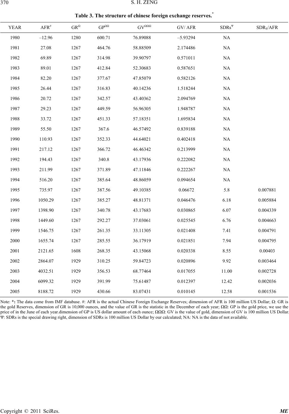 S. H. ZENG Copyright © 2011 SciRes. ME 370 Table 3. The structure of chinese foreign exchange reserves.* YEAR AFR# GRΩ GPΩΩ GVΩΩΩ GV/ AFR SDRsΨ SDRS/AFR 1980 –12.96 1280 600.71 76.89088 –5.93294 NA 1981 27.08 1267 464.76 58.88509 2.174486 NA 1982 69.89 1267 314.98 39.90797 0.571011 NA 1983 89.01 1267 412.84 52.30683 0.587651 NA 1984 82.20 1267 377.67 47.85079 0.582126 NA 1985 26.44 1267 316.83 40.14236 1.518244 NA 1986 20.72 1267 342.57 43.40362 2.094769 NA 1987 29.23 1267 449.59 56.96305 1.948787 NA 1988 33.72 1267 451.33 57.18351 1.695834 NA 1989 55.50 1267 367.6 46.57492 0.839188 NA 1990 110.93 1267 352.33 44.64021 0.402418 NA 1991 217.12 1267 366.72 46.46342 0.213999 NA 1992 194.43 1267 340.8 43.17936 0.222082 NA 1993 211.99 1267 371.89 47.11846 0.222267 NA 1994 516.20 1267 385.64 48.86059 0.094654 NA 1995 735.97 1267 387.56 49.10385 0.06672 5.8 0.007881 1996 1050.29 1267 385.27 48.81371 0.046476 6.18 0.005884 1997 1398.90 1267 340.78 43.17683 0.030865 6.07 0.004339 1998 1449.60 1267 292.27 37.03061 0.025545 6.76 0.004663 1999 1546.75 1267 261.35 33.11305 0.021408 7.41 0.004791 2000 1655.74 1267 285.55 36.17919 0.021851 7.94 0.004795 2001 2121.65 1608 268.35 43.15068 0.020338 8.55 0.00403 2002 2864.07 1929 310.25 59.84723 0.020896 9.92 0.003464 2003 4032.51 1929 356.53 68.77464 0.017055 11.00 0.002728 2004 6099.32 1929 391.99 75.61487 0.012397 12.42 0.002036 2005 8188.72 1929 430.66 83.07431 0.010145 12.58 0.001536 Note: *: The data come from IMF database. #: AFR is the actual Chinese Foreign Exchange Reserves; dimension of AFR is 100 million US Dollar; Ω: GR is the gold Reserves, dimension of GR is 10,000 ounces, and the value of GR is the statistic in the December of each year; ΩΩ: GP is the gold price, we use the price of in the June of each year.dimension of GP is US dollar amount of each ounce; ΩΩΩ: GV is the value of gold, dimension of GV is 100 million US Dollar. Ψ: SDRs is the special drawing right, dimension of SDRs is 100 million US Dollar by our calculated; NA: NA is the data of not available.
|