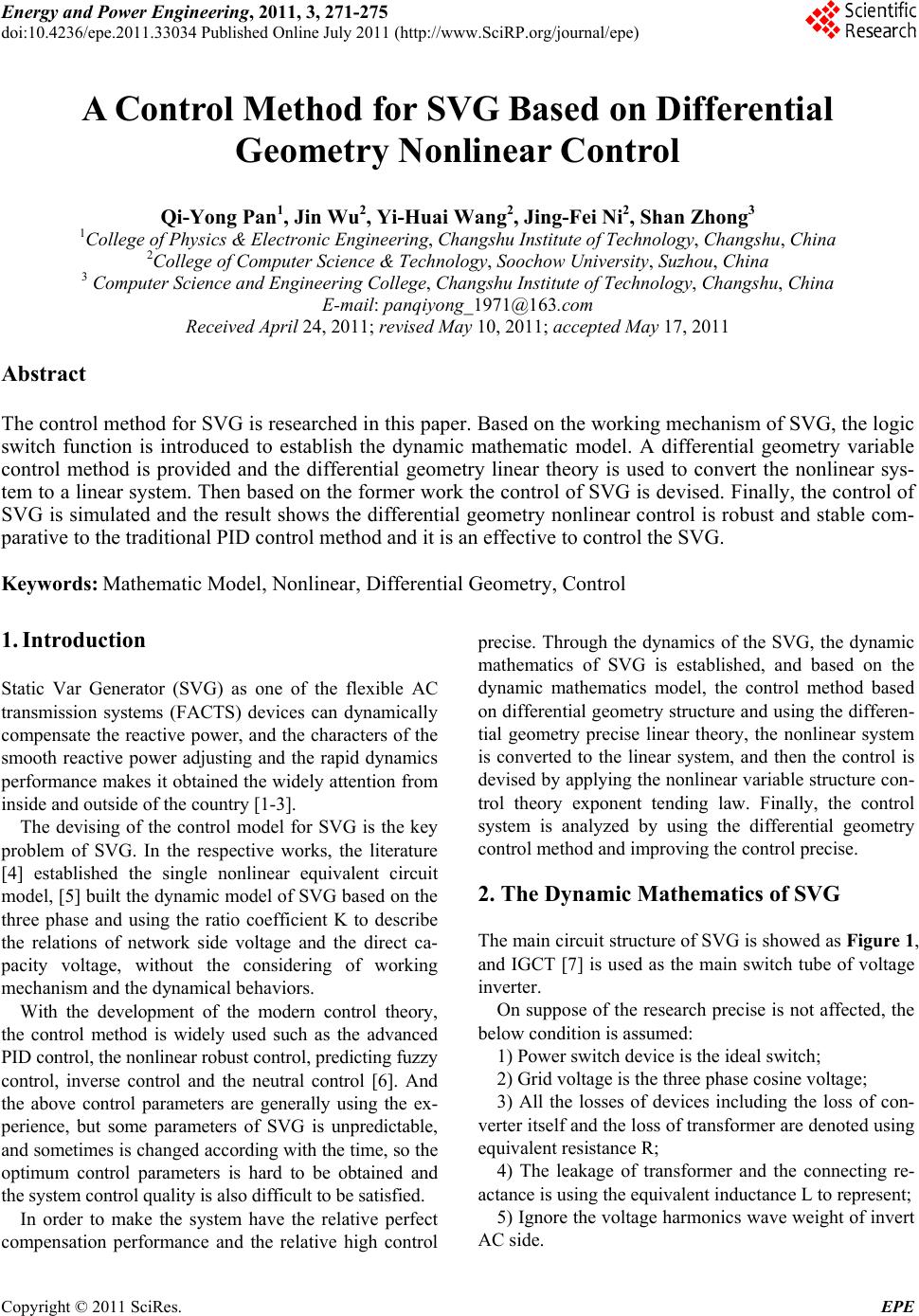Energy and Power En gi neering, 2011, 3, 271-275
doi:10.4236/epe.2011.33034 Published Online July 2011 (http://www.SciRP.org/journal/epe)
A Control Method for SVG Based on Differential
Geometry Nonlinear Control
Qi-Yong Pan1, Jin Wu2, Yi-Huai Wang2, Jing-Fei Ni2, Shan Zhong3
1College of Physics & Electronic Engineering, Changshu Institute of Technology, Changshu, China
2College of Computer Science & Technology, Soochow University, Suzhou, China
3 Computer Science and Engineering Colleg e, Changshu Institute of Technology, Changshu, China
Received April 24, 2011; revised May 10, 2011; accepted May 17, 2011
Abstract
The control method for SVG is researched in this paper. Based on the working mechanism of SVG, the logic
switch function is introduced to establish the dynamic mathematic model. A differential geometry variable
control method is provided and the differential geometry linear theory is used to convert the nonlinear sys-
tem to a linear system. Then based on the former work the control of SVG is devised. Finally, the control of
SVG is simulated and the result shows the differential geometry nonlinear control is robust and stable com-
parative to the traditional PID control method and it is an effective to control the SVG.
Keywords: Mathematic Model, Nonlinear, Differential Geometry, Control
1. Introduction
Static Var Generator (SVG) as one of the flexible AC
transmission systems (FACTS) devices can dynamically
compensate the reactive power, and the characters of the
smooth reactive power adjusting and the rapid dynamics
performance makes it obtained the widely attention from
inside and outside of the country [1-3].
The devising of the control model for SVG is the key
problem of SVG. In the respective works, the literature
[4] established the single nonlinear equivalent circuit
model, [5] built the dynamic model of SVG based on the
three phase and using the ratio coefficient K to describe
the relations of network side voltage and the direct ca-
pacity voltage, without the considering of working
mechanism and the dynamical behaviors.
With the development of the modern control theory,
the control method is widely used such as the advanced
PID control, the nonlinear robust control, predicting fuzzy
control, inverse control and the neutral control [6]. And
the above control parameters are generally using the ex-
perience, but some parameters of SVG is unpredictable,
and sometimes is changed according with the time, so the
optimum control parameters is hard to be obtained and
the system control quality is also difficult to be satisfied.
In order to make the system have the relative perfect
compensation performance and the relative high control
precise. Through the dynamics of the SVG, the dynamic
mathematics of SVG is established, and based on the
dynamic mathematics model, the control method based
on differential geometry structure and using the differen-
tial geometry precise linear theory, the nonlinear system
is converted to the linear system, and then the control is
devised by applying the nonlinear variable structure con-
trol theory exponent tending law. Finally, the control
system is analyzed by using the differential geometry
control method and improving the control precise.
2. The Dynamic Mathematics of SVG
The main circuit structure of SVG is showed as Figure 1,
and IGCT [7] is used as the main switch tube of voltage
inverter.
On suppose of the research precise is not affected, the
below condition is assumed:
1) Power switch device is the ideal switch;
2) Grid voltage is the three phase cosine voltage;
3) All the losses of devices including the loss of con-
verter itself and the loss of transformer are denoted using
equivalent resistance R;
4) The leakage of transformer and the connecting re-
actance is using the equivalent inductance L to represent;
5) Ignore the voltage harmonics wave weight of invert
AC side.

Q.-Y. PAN ET AL. 272
a
e
b
e
c
e
Figure 1. Circuit configuration of SVG.
The three-phase voltage is as Equation (1):
cos
2
cos π
3
2
cos π
3
a
abc bm
c
t
u
uuU t
u
t














 




 















(1)
In the Equation (1), is the max value of system
linear voltage.
m
U
The voltage of inverter AC side is showed as Equation
(2):

cos
22
cos π
33
2
cos π
3
a
abc bdc
c
t
e
ee Kut
e
t

















 



 














(2)
In Equation (2), where K is the ratio of inverter output
linear voltage with the direct current side voltage, and

is the phrase of device voltage and the system voltage.
In order to better analyze, the logic switch function
is introduced, the states of three bridge arm is using
a, b and c to represent, when the condition are
turning on the above bridge arm and turning off the be-
low bridge arm, the a, b and c are 1, and while
the condition are turning off the above bridge arm and
turning on the below bridge arm, the , and
are 0.
i
G
G GG
G GG
a
Gb Gc G
According to the Kirchhoff’s voltage law, the a-phase
loop equation is as Equation (3):

0
d
d
aaaNN
i
LRiuu
t 
a
u (3)
When a = 1 then0aNN ; while Guu0
a
G

then
. So Equation (2) can be written as bellow:
0
aN
u

0
d
d
aadcaN
i
LRiuGu
t 
a
u (4)
The b and c phase equation also can be obtained, as
for the three-phase input, there is no midline, so
0
abc
iii

, If the three phase power voltage is in
balance, then

0
1
3

N
abcd
uGGG c u (5)
The inverter is comprised of six power switch tubes
showed in Figure 1, and the on-off rule is as the same
bridge arm can be on at the same time.
Combined with the above switch function, the three
bridge arm just has two states as “1” and “0”.
1, 3 and 5
T forms eight models such as 000, 010,
011, 100, 101, 110 and 111. The switch model of 000
and 111 make the output voltage of invert as 0, so the
two switch models is at the state 0.
T T
The Kirchhoff current rule is applied in direct current
side capacitance positive node as Equation (6)
d
d
dc dc
dcaa bbcc
L
uu
CiGiGiG
tR
 (6)
For the circuit equation, it is very complex at the co-
ordinate at a, b and c, the d-q transform is used in the
equation of the three-phase voltage current, and the
transform matrix is showed as below:
22
cos cosπcos π
33
22
sin sinπsin π
33
22 2
22 2
tt t
Ctt t
 
 
2
3




 








 




 








(7)
Then the mathematics model of SVG in the coordinate
d-q is showed as Equation (8):
cos
dsin
d
cos sin0
1
0
0
d
q
dc
dc dc
dm
q
dc
RK
LL
iRK
i
tL
uKK
CC
iU
iL
u
L
















 













 
 

 
 
 
(8)
3. The Differential Geometry Nonlinear
Control of SVG
3.1. The Control Theory of Differential
Geometry for Nonlinear System
For the given multi-variable nonlinear system:

Q.-Y. PAN ET AL.273
i
 

1
,1,,
m
i
i
jj
X
fXgX u
y
hX jm










(9)
In the Equation (9),
X
is the local coordinate defined
on the n-dimension fluent
C
M
, and
are the vector field; is the mapping of C1
, ,,m fg g
h

in
M
as : h
j
M
R, and is the output. y
If i is the max positive integer satisfied the below
conditions, then
r
 
 
11
1
1
,,0,
,,0, 1,
ii
i
rr
gf igmf i
k k
gfigmfii i
LLhXLLhXX M
LLh XLLhXkrXM



 






(10)
In the Equation (10), is the

1
i
rfi
LhX
1
i
r

order
inverse derivative of i to

hX

f
X while
is the inverse derivative of

1
i
r
gm fi
LLhX



X
1
i
rfi
Lh

to vector field

g
X, where and

DX



EX are
showed as follows:

 
 
1
1
1 1
11 11
1 1
11
,,
,,
m
m
r r
gf gm
r r
gf mgmm
LLhXLL hX
DX
LLhX LLhX
 
 











1
1
m
rf
rfm
Lh X
EX
Lh X









Definition 1. The sufficient and necessary condition
for the decoupling of nonlinear system is the matrix
is non-singular, and the feedback control rule is
as follows:

DX
 
1
1
][uX XvDXEXDX 



 

v
(11)
So the system is decoupled on
M
showed as Equa-
tion (12)
  
 
,1,2,,
jj
X
fXgXx gXXv
yhXj m

 





 (12)
3.2. The Entire Linearizing of SVG
According to the Equation (8), the dynamic model of
SVG is the non-linear couple relation. Therefore, the
decoupling should be satisfied at first.
The state variable is defined as 1d
x
i, 2q
x
i

and
3dc
x
u, using

T
sin cosu


 yi to control the input,
at the same time using 1d and 2q as the out-
put. Therefore, the non-linear model of SVG can be rep-
resented as the affine non-linear forms:
yi
 


2
1
11
22
ii
i
X
fXgXu
yhX
yhX














(13)
In the Equation (13), where
 
12 3
12 3
33
0
0
0
dc dc
RK
x
xx
LL
RK
fXxx gXx
LL
KK
x
x
CC




 






 










The affine non-linear system such as Equation (9),
according to the Equation (10), the below equations can
be obtained:


110
g
LhX ;


210
g
LhX;

11fR
Lh Xxx
L2

 ;

113gf
K
LLh Xx
L
;

213gf dc
K
LLhXx
C
 ;


210
g
LhX;


220
g
Lh X;

21fR
Lh Xxx
L
  2 ;

123gf
K
LLhXx
L
 ;

223gf dc
K
LLhXx
C
 ;
From the above equations we can know the matrix


DX is not singular and satisfying the conditions for
decoupling of input and output.
The state equations on the new coordinate are as bel-
lows:
 
 
12
11
22
11 1
12
22
22
22 2
fgf
fgf
zz
zLhXLLhXu
zz
zLhX LLhXu















(14)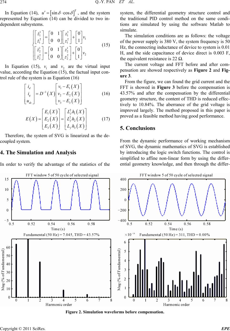

Q.-Y. PAN ET AL. 274

In Equation (14),

T
sin cosu


 , and the system
represented by Equation (14) can be divided to two in-
dependent subsystems.
system, the differential geometry structure control and
the traditional PID control method on the same condi-
tions are simulated by using the software Matlab to
simulate.
11
11
1
22
11
11
22
2
22
22
01 0
001
01 0
001
zz
v
zz
zz
v
zz
 
 

 
 
 
  
 
 

 
 

 





(15)
The simulation conditions are as follows: the voltage
of the power supply is 380 V, the system frequency is 50
Hz, the connecting inductance of device to system is 0.01
H, and the side capacitance of device direct is 0.003 F,
the equivalent resistance is 22 Ω.
The current voltage and FFT before and after com-
pensation are showed respectively as Figure 2 and Fig-
ure 3.
In Equation (15), 1 and 2 are the virtual input
value, according the Equation (15), the factual input con-
trol rule of the system is as Equation (16)
v v
From the figure, we can found the grid current and the
FFT is showed in Figure 3 before the compensation is
43.57% and after the compensation by the differential
geometry structure, the content of THD is reduced effec-
tively to 10.84%. The aberrance of the grid voltage is
improved largely. The method proposed in this paper is
proved as a feasible method having good performance.




11
1
22
33
d
q
dc
ivE
iDXvEX
uvE

 
 



 
 
 
X
X




(16)







2
11
2
22
33
f
f
f
EX LhX
EXEXLh X
EX LhX











(17)
5. Conclusions
Therefore, the system of SVG is linearized as the de-
coupled system. From the dynamic performance of working mechanism
of SVG, the dynamic mathematics of SVG is established
by introducing the logic switch functions. The control is
simplified to affine non-linear form by using the differ-
ential geometry knowledge, and then through the differ-
4. The Simulation and Analysis
In order to verify the advantage of the statistics of the
Figure 2. Simulation waveforms before compensation.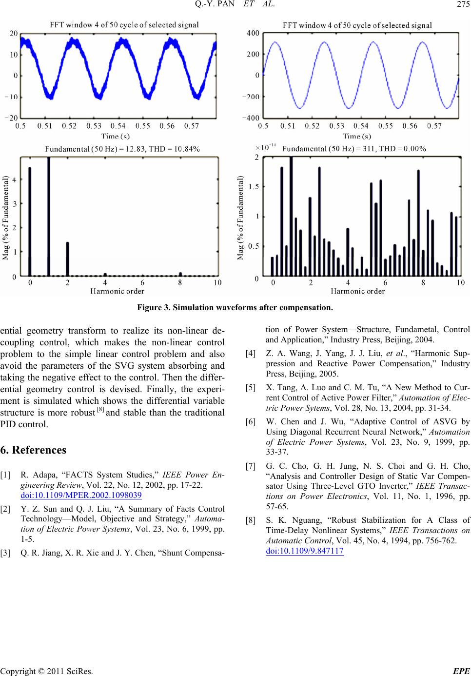

Q.-Y. PAN ET AL.275
Figure 3. Simulation waveforms after compensation.
ential geometry transform to realize its non-linear de-
coupling control, which makes the non-linear control
problem to the simple linear control problem and also
avoid the parameters of the SVG system absorbing and
taking the negative effect to the control. Then the differ-
ential geometry control is devised. Finally, the experi-
ment is simulated which shows the differential variable
structure is more robust [8] and stable than the traditional
PID control.
6. References
[1] R. Adapa, “FACTS System Studies,” IEEE Power En-
gineering Review, Vol. 22, No. 12, 2002, pp. 17-22.
doi:10.1109/MPER.2002.1098039
[2] Y. Z. Sun and Q. J. Liu, “A Summary of Facts Control
Technology—Model, Objective and Strategy,” Automa-
tion of Electric Power Systems, Vol. 23, No. 6, 1999, pp.
1-5.
[3] Q. R. Jiang, X. R. Xie and J. Y. Chen, “Shunt Compensa-
tion of Power System—Structure, Fundametal, Control
and Application,” Industry Press, Beijing, 2004.
[4] Z. A. Wang, J. Yang, J. J. Liu, et al., “Harmonic Sup-
pression and Reactive Power Compensation,” Industry
Press, Beijing, 2005.
[5] X. Tang, A. Luo and C. M. Tu, “A New Method to Cur-
rent Control of Active Power Filter,” Automation of Elec-
tric Power Sytems, Vol. 28, No. 13, 2004, pp. 31-34.
[6] W. Chen and J. Wu, “Adaptive Control of ASVG by
Using Diagonal Recurrent Neural Network,” Automation
of Electric Power Systems, Vol. 23, No. 9, 1999, pp.
33-37.
[7] G. C. Cho, G. H. Jung, N. S. Choi and G. H. Cho,
“Analysis and Controller Design of Static Var Compen-
sator Using Three-Level GTO Inverter,” IEEE Transac-
tions on Power Electronics, Vol. 11, No. 1, 1996, pp.
57-65.
[8] S. K. Nguang, “Robust Stabilization for A Class of
Time-Delay Nonlinear Systems,” IEEE Transactions on
Automatic Control, Vol. 45, No. 4, 1994, pp. 756-762.
doi:10.1109/9.847117