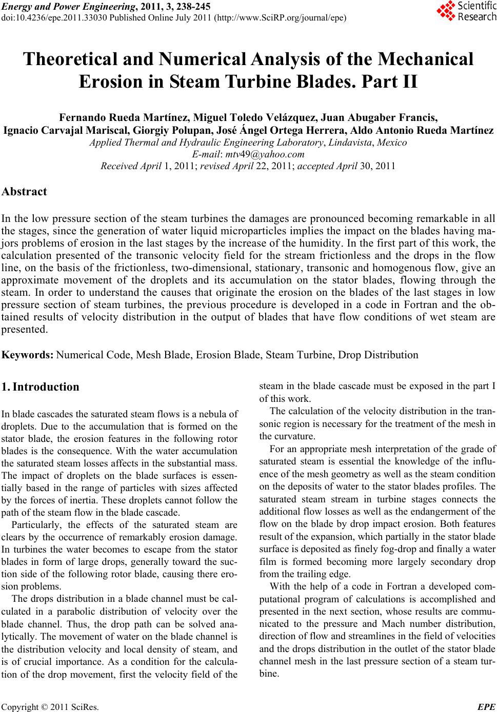Energy and Power Engineering, 2011, 3, 238-245
doi:10.4236/epe.2011.33030 Published Online July 2011 (http://www.SciRP.org/journal/epe)
Theoretical and Numerical Analysis of the Mechanical
Erosion in Steam Turbine Blades. Part II
Fernando Rueda Martínez, Miguel Toledo Velázquez, Juan Abugaber Francis,
Ignacio Carvajal Mariscal, Giorgiy Polupan, José Ángel Ortega Herrera, Aldo Antonio Rueda Martínez
Applied Thermal and Hydraulic Engineering Laboratory, Lindavista, Mexico
Received April 1, 2011; revised April 22, 2011; accepted April 30, 2011
Abstract
In the low pressure section of the steam turbines the damages are pronounced becoming remarkable in all
the stages, since the generation of water liquid microparticles implies the impact on the blades having ma-
jors problems of erosion in the last stages by the increase of the humidity. In the first part of this work, the
calculation presented of the transonic velocity field for the stream frictionless and the drops in the flow
line, on the basis of the frictionless, two-dimensional, stationary, transonic and homogenous flow, give an
approximate movement of the droplets and its accumulation on the stator blades, flowing through the
steam. In order to understand the causes that originate the erosion on the blades of the last stages in low
pressure section of steam turbines, the previous procedure is developed in a code in Fortran and the ob-
tained results of velocity distribution in the output of blades that have flow conditions of wet steam are
presented.
Keywords: Numerical Code, Mesh Blade, Erosion Blade, Steam Turbine, Drop Distribution
1. Introduction
In blade cascades the saturated steam flows is a nebula of
droplets. Due to the accumulation that is formed on the
stator blade, the erosion features in the following rotor
blades is the consequence. With the water accumulation
the saturated steam losses affects in the substantial mass.
The impact of droplets on the blade surfaces is essen-
tially based in the range of particles with sizes affected
by the forces of inertia. These droplets cannot follow the
path of the steam flow in the blade cascade.
Particularly, the effects of the saturated steam are
clears by the occurrence of remarkably erosion damage.
In turbines the water becomes to escape from the stator
blades in form of large drops, generally toward the suc-
tion side of the following rotor blade, causing there ero-
sion problems.
The drops distribution in a blade channel must be cal-
culated in a parabolic distribution of velocity over the
blade channel. Thus, the drop path can be solved ana-
lytically. The movement of water on the blade channel is
the distribution velocity and local density of steam, and
is of crucial importance. As a condition for the calcula-
tion of the drop movement, first the velocity field of the
steam in the blade cascade must be exposed in the part I
of this work.
The calculation of the velocity distribution in the tran-
sonic region is necessary for the treatment of the mesh in
the curvature.
For an appropriate mesh interpretation of the grade of
saturated steam is essential the knowledge of the influ-
ence of the mesh geometry as well as the steam condition
on the deposits of water to the stator blades profiles. The
saturated steam stream in turbine stages connects the
additional flow losses as well as the endangerment of the
flow on the blade by drop impact erosion. Both features
result of the expansion, which partially in the stator blade
surface is deposited as finely fog-drop and finally a water
film is formed becoming more largely secondary drop
from the trailing edge.
With the help of a code in Fortran a developed com-
putational program of calculations is accomplished and
presented in the next section, whose results are commu-
nicated to the pressure and Mach number distribution,
direction of flow and streamlines in the field of velocities
and the drops distribution in the outlet of the stator blade
channel mesh in the last pressure section of a steam tur-
bine.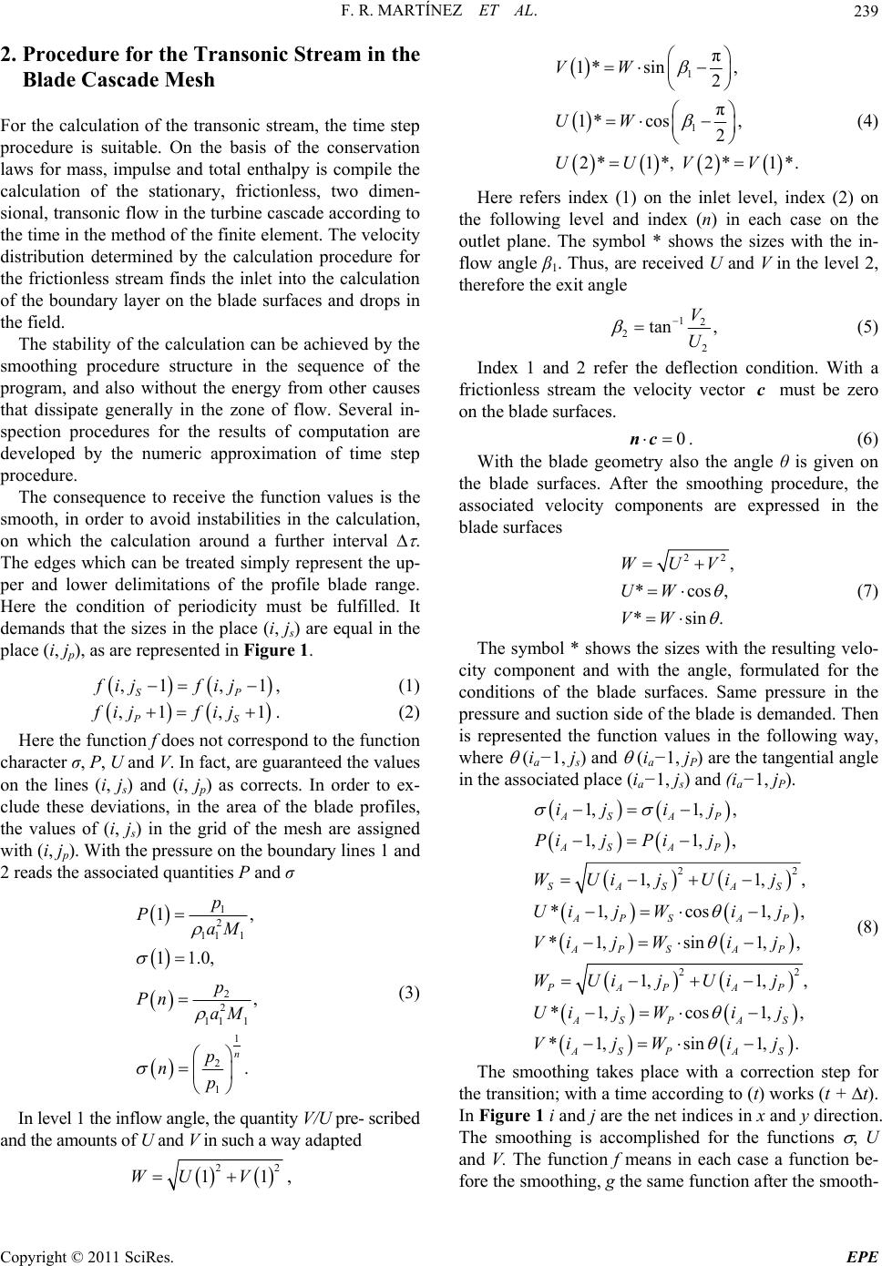

F. R. MARTÍNEZ ET AL.239

P
 
,1 ,1
S
fij fij 
2. Procedure for the Transonic Stream in the
Blade Cascade Mesh
For the calculation of the transonic stream, the time step
procedure is suitable. On the basis of the conservation
laws for mass, impulse and total enthalpy is compile the
calculation of the stationary, frictionless, two dimen-
sional, transonic flow in the turbine cascade according to
the time in the method of the finite element. The velocity
distribution determined by the calculation procedure for
the frictionless stream finds the inlet into the calculation
of the boundary layer on the blade surfaces and drops in
the field.
The stability of the calculation can be achieved by the
smoothing procedure structure in the sequence of the
program, and also without the energy from other causes
that dissipate generally in the zone of flow. Several in-
spection procedures for the results of computation are
developed by the numeric approximation of time step
procedure.
The consequence to receive the function values is the
smooth, in order to avoid instabilities in the calculation,
on which the calculation around a further interval 
 .
The edges which can be treated simply represent the up-
per and lower delimitations of the profile blade range.
Here the condition of periodicity must be fulfilled. It
demands that the sizes in the place (i, js) are equal in the
place (i, jp), as are represented in Figure 1.
 
,1 ,1
S
fij fij , (1)
P. (2)
Here the function f does not correspond to the function
character σ, P, U and V. In fact, are guaranteed the values
on the lines (i, j
s) and (i, j p) as corrects. In order to ex-
clude these deviations, in the area of the blade profiles,
the values of (i, js) in the grid of the mesh are assigned
with (i, jp). With the pressure on the boundary lines 1 and
2 reads the associated quantities P and σ




1
2
11 1
2
2
11 1
1
2
1
1,
11.0,
,
.
n
p
PaM
p
Pn aM
p
np










(3)
In level 1 the inflow angle, the quantity V/U pre- scribed
and the amounts of U and V in such a way adapted
 
22
11WU V ,


 
1
1
π
1* sin,
2
π
1* cos,
2
2*1*, 2*1*.
VW
UW
UUVV



 



 



(4)
Here refers index (1) on the inlet level, index (2) on
the following level and index (n) in each case on the
outlet plane. The symbol * shows the sizes with the in-
flow angle β1. Thus, are received U and V in the level 2,
therefore the exit angle
12
2
2
tan ,
V
U


 (5)
Index 1 and 2 refer the deflection condition. With a
frictionless stream the velocity vector must be zero
on the blade surfaces.
c
0

nc . (6)
With the blade geometry also the angle θ is given on
the blade surfaces. After the smoothing procedure, the
associated velocity components are expressed in the
blade surfaces
22
,
*cos
*sin.
WUV
UW
VW
,





(7)
The symbol * shows the sizes with the resulting velo-
city component and with the angle, formulated for the
conditions of the blade surfaces. Same pressure in the
pressure and suction side of the blade is demanded. Then
is represented the function values in the following way,
where
 (ia−1, js) and  (ia−1, jP) are the tangential angle
in the associated place (ia−1, js) and (ia−1, jP).




 

 
 

 
 
22
22
1,1, ,
1,1, ,
1,1, ,
*1,cos 1,
*1,sin 1,,
1,1, ,
*1,cos 1,
*1,sin 1,.
AS AP
AS AP
SASAS
AP SAP
AP SAP
PAPAP
AS PAS
AS PAS
ij ij
Pi jPi j
WUi jUi j
Ui jWi j
Vi jWi j
WUijUi j
Ui jWi j
Vi jWij








 
 


 

,
,
(8)
The smoothing takes place with a correction step for
the transition; with a time according to (t) works (t + t).
In Figure 1 i and j are the net indices in x and y direction.
The smoothing is accomplished for the functions
 , U
and V. The function f means in each case a function be-
fore the smoothing, g the same function after the smooth-

F. R. MARTÍNEZ ET AL. 240
Figure 1. Designation of mesh for the zone of flow.
ing and according to the exactitude of the calculation it
can be selected the size of
 , which is adapted to the de-
sired computational accuracy.
 




,, 1, 1,
,1,14
g
ijfij fijfij
fij fij


  

  

(9)
For a two-dimensional computing area the permissible
border for the time step size Δt
22
11
1,
y
xc
c
ta
xy xy


 

 

(10)
a is the local speed sound. The computer cost depends of
the time step size above t. The organization of a more
finely mesh, t must be selected smaller, in order to se-
cure stability. The smoothing absorbs practically the rip-
ples of the solution functions resulted from computing
inaccuracies. In this case a polynomial of two degrees
calculated according to the method of the difference
squares is used. A simplification of the equation system
is possible by introduction of a constant specific total
enthalpy for the entire computing area. This is from the
first law of thermodynamic with open stationary system
and taking or adding work. The energy equation in dif-
ferential form can be replaced therefore by
3.5 for air 1.4
1
tot tot
RR RR
hh
pp

 





 . (11)
In the proximity of the surface of the wet body the
drop movement is affected by the velocity profile of the
boundary layer. The integral condition for the impulse as
the force equilibrium in x-direction, averaged over the
boundary layer thickness δ:
2 21
2
2
dd d20
d
f
c
ux
M
xu






 


2
(12)
with the definitions
1
0
1
uy
u









2
0
1d
uu
y
uu

 






: Pulse loss thickness. (13b)
2:
2
fw
c

u


  Friction coefficient. (14)



:
ux
Max



 Local Mach number. (15)
The local speed sound aδ(x) is according gas dynamics
laws from the speed uδ(x) and Mδ(x). The integral condi-
tion is kept for the kinematic energy
2
34
3
3
d32 0
dD
Mc
x





 


(16)
with the definition
2
301d
uu
y
uu

 










: Loss of energy thickness.
(17)
401d:
uy
u


 




 


Density loss thickness. (18)
3
0
1d:
12
u
D
c
u




u

Integral of dissipations. (19)
121 2
H



and 323 2 H

 . (20)
In order to calculate the impact of drops on blade pro-
files is necessary to describe the movement of drops in a
zone of flow. The general beginning for the calculation
of an unsteady drop movement proceeds from the force
equilibrium:
0

K. (21)
The sum of all forces around a drop is zero. The Equa-
tion (21) lead to the relationship
0

WT . (22)
where the strength becomes


2
2π
Wrelrel
cww 
T
r

W, (23)
and the force of inertia is
dd
TT
mwt

T. (24)
Here cw is the coefficient of drag, ρ is the steam den-
sity, rT the drop radius and wrel the relative velocity
between steam and drop in accordance with
relD T

www. (25)
The drop mass mT is calculated


3
43π
T
m 
TT
r

 (26)
Then, the general differential equation for drop move-
ment


2
dd 2π
TTWrelrelT
mtc w  r

ww, (27)
d: Displacement thickness. (13a)
the drops with a spherical shae are due to the force by the p

F. R. MARTÍNEZ ET AL.241

surface tension. For the calculation of drop courses the
velocity field must be given by drops moving with the
help of the Equiation (27). The amount of relative velocity


2
2
rel DxDy
wwxwy

, (28)
where the steam flow in the place (x, y) by the velocities
wDx and wDy is given, following the relationship of the
Equation (25) of the equation system: ψ



Re
83 0
T
TT crelDx w
rxcfw wx  
 , (29)



Re
83 0
T
TT crelDy w
rycfw wy  
 .(30)
The momentary position x(i) and y(i, j) of the drop is
admitted from the Equations (29) and (30). Index i and j
refers to the x and y direction. The droplet impact on the
blade surface is essentially based in the range of particles
with sizes affected by the forces of inertia. These drop-
lets cannot follow the stream of the steam flow, as is
showed in Figure 2 by the courses ,Ti

and ,1Ti


(remarked lines) in the blade channel. These large drop-
lets become to escape from the stator blades, generally
toward the suction side of the following rotor blade,
causing there erosion problems. The drop distribution in
the mesh outlet level is represented on the basis of a
fundamental flow pattern in a blade channel. It provides
that the drops before the mesh are homogeneous distrib-
uted and that the drop velocity and steam velocity are
identical to cTO and cDO here. The stream condition con-
tinues homogeneous by p0 and Y0. The drop radius is rT0.
Between the two drop courses ,Ti

and ,1Ti


in the
distance Δt0, i, which are identical to the steam stream-
lines in the mesh and two surfaces parallel to the indica-
tion level Δt0,1, the water mass flow is
0,0 0,Ti i
mYm

, (31)
whereby 0, i is the total mass stream between the
streamlines and Y0 is the moisture content in the inlet.
The number of drops in the flow is then
m

0,
0, 3
0
4π
3
Ti
i
T
m
n
r





. (32)
A certain part of drops which flow between the pres-
sure side of the blade enter in contact with the profile, all
these drops are closed strongly in a very thin layer on the
profile surface and are concentrated finally along the
flow in a narrow volume of the trailing edge, forming a
water film.
The remaining drops leave from the mesh with a ve-
locity which deviates in size and direction from the local
steam velocity. In addition, they are distributed irregularly
larly over the division. The quantity of water between the
two drop courses in the level 1 is
Figure 2. Nomenclature for the moisture distribution in the
mesh outlet plane.


3
1,1,1 1
43π
Ti iT
mnr




 (33)
The mid drop course in the steam flow between the
courses ,Ti

and ,1Ti


in level 1 is:

1,1 1,1,1,1,1,
sin cos
D
iDiDiiTiD
mc t  

 
i (34)
Steam has a medium velocity 1,
D
i
c in the level 1.
This direction is given by 1, .
D
i

The term


1, 1,
cos Ti Di   of the steam quantity is referred to the
drop course direction.
3. Particular Characteristics
The steam turbine that was used in this study gives a
power of 300 MW and is analyzed a rotor blade in the
last stage. The turbine is working in a thermoelectric
plant of CFE installed in Estado de México, México.
With real, ideal and design a value of operation [1], a
graphic of steam expansion is obtained over the diagram
of Mollier observed in the Fi g ure 3.
The low pressure section of the steam turbine has five
stages. The row of rotor step consists of 65 working
blades with a measurement of 716 ± 0.5 mm each one;
the profile of the rotor blade to treat is 1182SGAx and
the δdesp cavities on the different large of the blades
measured directly over the affected zone are referred in
Figure 4. The measurements were 30 mm for the base,
23 mm for the middle zone and 18 for the peripherical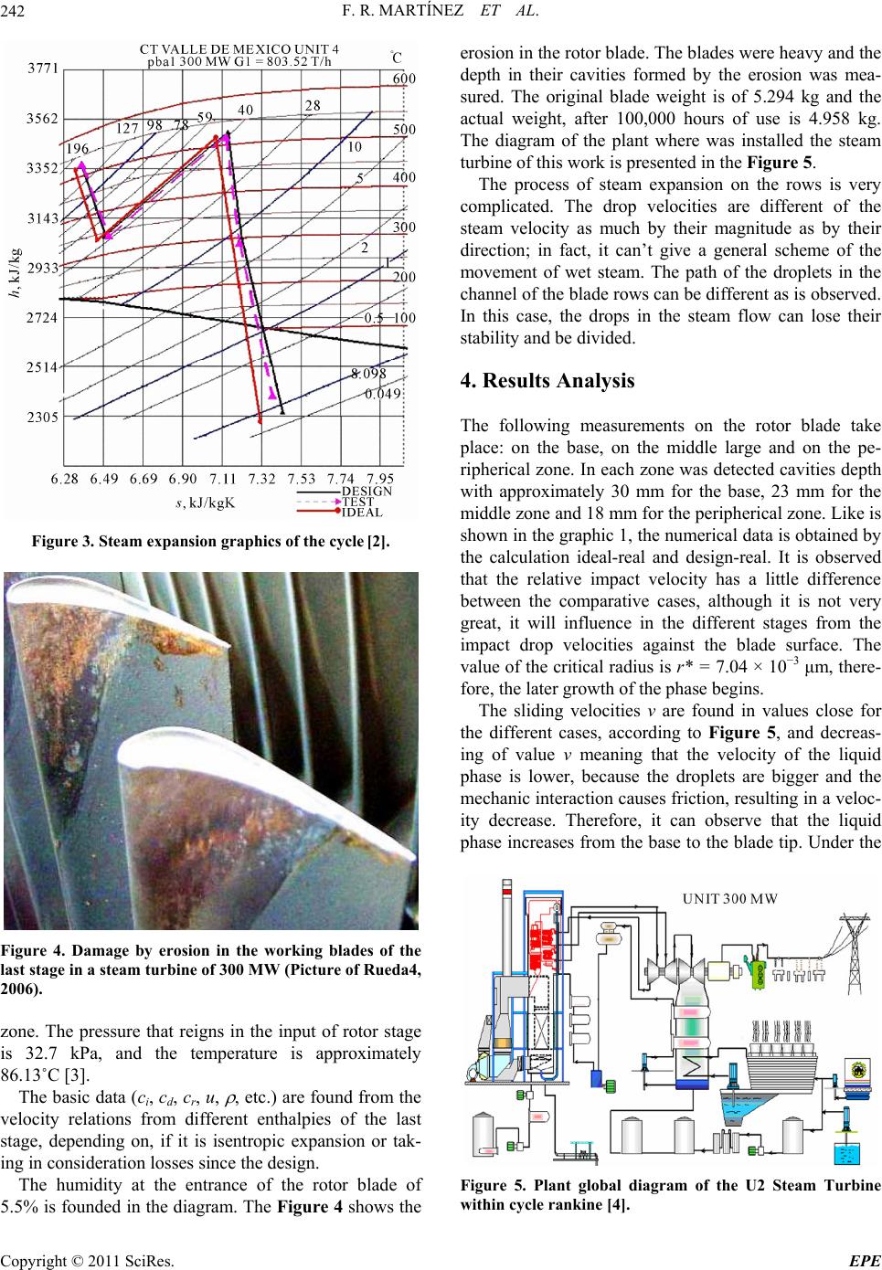

F. R. MARTÍNEZ ET AL. 242
Figure 3. Steam expansion graphic s of the cycle [2].
Figure 4. Damage by erosion in the working blades of the
last stage in a steam turbine of 300 MW (Picture of Rueda4,
2006).
zone. The pressure that reigns in the input of rotor stage
is 32.7 kPa, and the temperature is approximately
86.13˚C [3].
The basic data (ci, cd, cr, u,  , etc.) are found from the
velocity relations from different enthalpies of the last
stage, depending on, if it is isentropic expansion or tak-
ing in consideration losses since the design.
The humidity at the entrance of the rotor blade of
5.5% is founded in the diagram. The Figure 4 shows the
erosion in the rotor blade. The blades were heavy and the
depth in their cavities formed by the erosion was mea-
sured. The original blade weight is of 5.294 kg and the
actual weight, after 100,000 hours of use is 4.958 kg.
The diagram of the plant where was installed the steam
turbine of this work is presented in the Figure 5.
The process of steam expansion on the rows is very
complicated. The drop velocities are different of the
steam velocity as much by their magnitude as by their
direction; in fact, it can’t give a general scheme of the
movement of wet steam. The path of the droplets in the
channel of the blade rows can be different as is observed.
In this case, the drops in the steam flow can lose their
stability and be divided.
4. Results Analysis
The following measurements on the rotor blade take
place: on the base, on the middle large and on the pe-
ripherical zone. In each zone was detected cavities depth
with approximately 30 mm for the base, 23 mm for the
middle zone and 18 mm for the peripherical zone. Like is
shown in the graphic 1, the numerical data is obtained by
the calculation ideal-real and design-real. It is observed
that the relative impact velocity has a little difference
between the comparative cases, although it is not very
great, it will influence in the different stages from the
impact drop velocities against the blade surface. The
value of the critical radius is r* = 7.04 × 10−3 μm, there-
fore, the later growth of the phase begins.
The sliding velocities v are found in values close for
the different cases, according to Figure 5, and decreas-
ing of value v meaning that the velocity of the liquid
phase is lower, because the droplets are bigger and the
mechanic interaction causes friction, resulting in a veloc-
ity decrease. Therefore, it can observe that the liquid
phase increases from the base to the blade tip. Under the
Figure 5. Plant global diagram of the U2 Steam Turbine
within cycle rankine [4].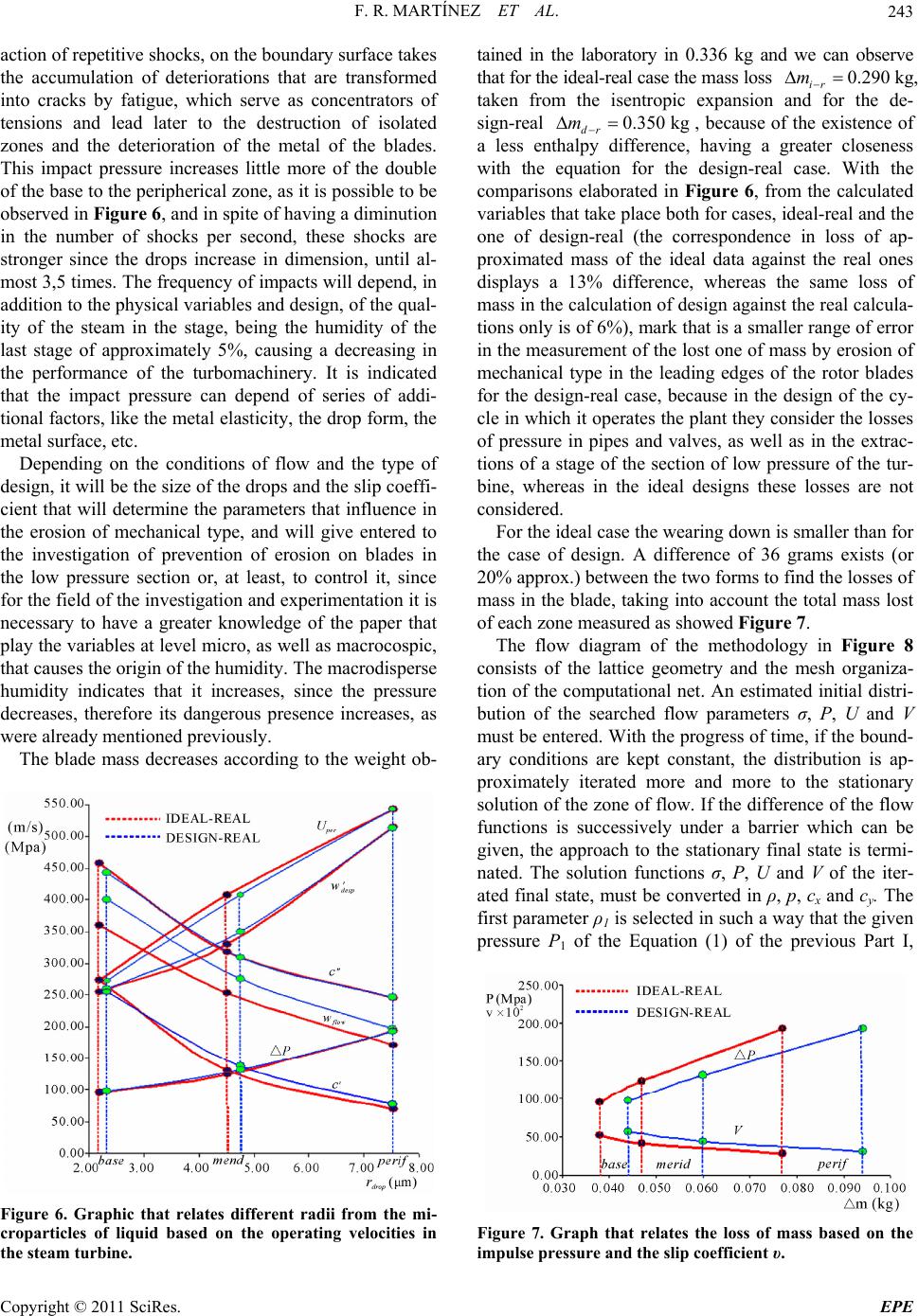

F. R. MARTÍNEZ ET AL.243
action of repetitive shocks, on the boundary surface takes
the accumulation of deteriorations that are transformed
into cracks by fatigue, which serve as concentrators of
tensions and lead later to the destruction of isolated
zones and the deterioration of the metal of the blades.
This impact pressure increases little more of the double
of the base to the peripherical zone, as it is possible to be
observed in Figure 6, and in spite of having a diminution
in the number of shocks per second, these shocks are
stronger since the drops increase in dimension, until al-
most 3,5 times. The frequency of impacts will depend, in
addition to the physical variables and design, of the qual-
ity of the steam in the stage, being the humidity of the
last stage of approximately 5%, causing a decreasing in
the performance of the turbomachinery. It is indicated
that the impact pressure can depend of series of addi-
tional factors, like the metal elasticity, the drop form, the
metal surface, etc.
Depending on the conditions of flow and the type of
design, it will be the size of the drops and the slip coeffi-
cient that will determine the parameters that influence in
the erosion of mechanical type, and will give entered to
the investigation of prevention of erosion on blades in
the low pressure section or, at least, to control it, since
for the field of the investigation and experimentation it is
necessary to have a greater knowledge of the paper that
play the variables at level micro, as well as macrocospic,
that causes the origin of the humidity. The macrodisperse
humidity indicates that it increases, since the pressure
decreases, therefore its dangerous presence increases, as
were already mentioned previously.
The blade mass decreases according to the weight ob-
Figure 6. Graphic that relates different radii from the mi-
croparticles of liquid based on the operating velocities in
the steam turbine.
tained in the laboratory in 0.336 kg and we can observe
that for the ideal-real case the mass loss kg,
taken from the isentropic expansion and for the de-
sign-real
0.290
ir
m 
0.350 kg
dr
m

, because of the existence of
a less enthalpy difference, having a greater closeness
with the equation for the design-real case. With the
comparisons elaborated in Figure 6, from the calculated
variables that take place both for cases, ideal-real and the
one of design-real (the correspondence in loss of ap-
proximated mass of the ideal data against the real ones
displays a 13% difference, whereas the same loss of
mass in the calculation of design against the real calcula-
tions only is of 6%), mark that is a smaller range of error
in the measurement of the lost one of mass by erosion of
mechanical type in the leading edges of the rotor blades
for the design-real case, because in the design of the cy-
cle in which it operates the plant they consider the losses
of pressure in pipes and valves, as well as in the extrac-
tions of a stage of the section of low pressure of the tur-
bine, whereas in the ideal designs these losses are not
considered.
For the ideal case the wearing down is smaller than for
the case of design. A difference of 36 grams exists (or
20% approx.) between the two forms to find the losses of
mass in the blade, taking into account the total mass lost
of each zone measured as showed Figure 7.
The flow diagram of the methodology in Figure 8
consists of the lattice geometry and the mesh organiza-
tion of the computational net. An estimated initial distri-
bution of the searched flow parameters σ, P, U and V
must be entered. With the progress of time, if the bound-
ary conditions are kept constant, the distribution is ap-
proximately iterated more and more to the stationary
solution of the zone of flow. If the difference of the flow
functions is successively under a barrier which can be
given, the approach to the stationary final state is termi-
nated. The solution functions σ, P, U and V of the iter-
ated final state, must be converted in ρ, p, cx and cy. The
first parameter ρ1 is selected in such a way that the given
pressure P1 of the Equation (1) of the previous Part I,
Figure 7. Graph that relates the loss of mass based on the
impulse pressure and the slip coefficient υ.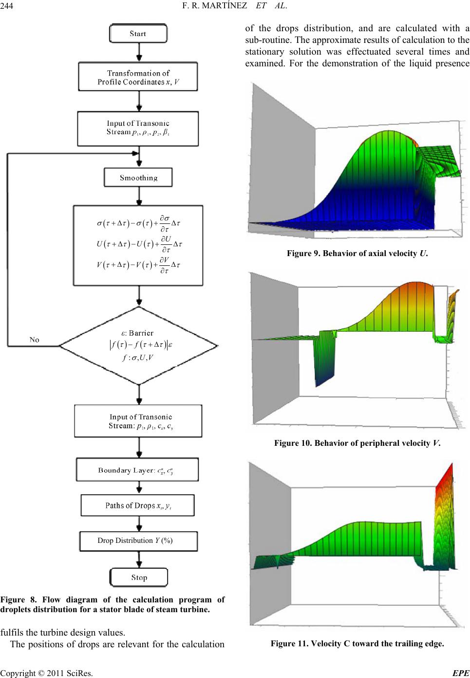

F. R. MARTÍNEZ ET AL. 244



U
UU
V
VV


 


 


 


 


 


 

 
:,,
ff
fUV




Drop Distribution Y (%)
Figure 8. Flow diagram of the calculation program of
droplets distribution for a stator blade of steam turbine.
fulfils the turbine design values.
The positions of drops are relevant for the calculation
of the drops distribution, and are calculated with a
sub-routine. The approximate results of calculation to the
stationary solution was effectuated several times and
examined. For the demonstration of the liquid presence
Figure 9. Behavior of axial velocity U.
Figure 10. Behavior of peripheral velocity V.
Figure 11. Velocity C toward the trailing edge.

F. R. MARTÍNEZ ET AL. 245
Figure 12. Inlet to exit Mach number in blade channel.
influence, a calculation with the polytropic efficiency is
presented.
The results in Figures 9 to 12 are showed. In the fig-
ures it can observe a spontaneous condensation that de-
celerated the Mach, axial and absolute velocity in the
outlet blade channel, being the large secondary drops in
the saturated steam stream are essentially responsible by
the negative consequences.
The proceeding for a stator blade mesh by systematic
deformations for transonic flow conditions, with respect
to smaller drops of water, is introduced. Being the liquid
impact erosion a major technological problem in steam
turbines, the interaction of drops, droplets or clusters,
plays an important role in the low pressure section. The
erosion that appears on the blades by the repetitive impact
of the great droplets causes damages in the surface of
them and, therefore, changes in the flow conditions of the
stage. For an appropriate mesh configuration of the grade
of saturated steam is essential the knowledge of influence
of the mesh geometry and the steam condition on the de-
posits of water to the stator blades profiles. With a devel-
oped code in Fortran, the calculations of drops distribu-
tion in the outlet of the stator blade mesh can be accom-
plished. The available information to contribute in the
knowledge of the understanding of the drops distribution
in the outlet stator blade mesh is analyzed.
5. Conclusions
The entire work provides information about formation
and humidity distribution, as well as an evaluation with
the existing theoretical treatment through a numerical
development. The solutions obtained by means of the
schemes of finite element show that the greater percent-
age of humidity begins to give when coming out of the
throat of the channel, generally in the change of curva-
ure radio of the surface of suction of the profile. Due to
this humidity concentration the properties of the fluid,
the flow angle and the Mach number when coming out of
the channel differ from those cascades of blades that
work with superheated steam.
In the flow channel, the drops that conform the humid-
ity are turned aside of the trajectories of the streamlines,
this is due to the inertia forces that increase while the
size of the drop is greater. It is in the side of pressure of
the blade stator where the greater amount of drops is
concentrated, these crosses through the cascade which
will be accumulated and been forming a water film on
the surface.
The obtained percentage of humidity increases at the
outlet of the cascade, this drift that the process of accu-
mulation of drops in the blade stator be continuous, the
film that forms will be broken and greater drops will
affect the edge of entrance of the rotor blade following
by the suction side.
The increase in the amount of humidity is translated in
losses that will become evident after certain running
hours from the turbine and they will be reflected in his
operation. To understand the phenomenon of erosion like
a problem that is derived from the humidity existing in
the channel of flow and accumulated in the stator blade,
it allows improving the efficiency of the steam turbines
until in an 8%.
This data is excellent to define the amount of humidity,
that remains in the channel, deposited in the form of liq-
uid film, and take the necessary measures from preven-
tion and maintenance with respect to the problem of the
erosion that arises by that reason.
6. References
[1] “Closing report of Tests of Evaluation,” Technical Sub-
division, Department of Evaluations of Processes, Office
of Thermal Systems, CTM-VM, CFE, October 2003.
[2] M. F. Rueda, V. M. Toledo, S. F. Sánchez and H. J. A.
Ortega, “Analysis of Erosion by Nucleation in a Steam
Turbine of 300 MW,” The 2nd International Simposium
on Energy Engineering, Economics and Policy, Florida,
29 June-2 July 2010, p. 5.
[3] “Handbook of Engineering Datas,” Technical Subdivi-
sion, Department of Evaluations of Processes, Office of
Thermal Systems, CTM-VM, CFE, 1980, p. 39.
[4] M. F. Rueda, V. M. Toledo, S. F. Sánchez, G. Polupan, M.
A. A. Rueda and L. G. Jarquín, “Review of Nucleation
Phenomena in Steam Turbines,” V Congreso Internacional
de Ingeniería Electromecánica y de Sistemas, MEC100,
Instituto Politécnico Nacional, México, D. F., 2008.
[5] J. B. Young, “Wet Steam Research at Cambridge 1980-
1985,” EPRI Workshop on Moisture Nucleation in Steam
Turbines, October 1995, pp. 11-13.
t