Modern Economy, 2011, 2, 308-323
doi:10.4236/me.2011.23034 Published Online July2011 (http://www.SciRP.org/journal/me)
Determinants and Prevalence of Rural Poverty in West,
East and Southern African Countries
Joachim Nyemeck Binam1*, Judith Oduol2, Luke Olarinde1, Aliou Diagne3, Ad e w al e Adekunl e 4
1Forum for Agricultural Research in Africa (FARA) Sub-Saharan Africa Challenge Program (SSA CP) KKM
PLS-IAR-Agric Research Station (ARS), Kano, Nigeria
2Forum for Agricultural Research in Africa (FARA), Kachwekano Zonal Agricultural Research and
Development Institute, Kabale, Uganda
3Africa Rice Center (AfricaRice), Cotonou, Benin
4Cantonments, Forum for Agricultural Research in Africa (FARA), Accra, Ghana
Received February 09, 2011; revised April 3, 2011; accepted April 15, 2011
Abstract
In this paper, we determine the extent to which the variation in poverty incidence can be explained by insti-
tutional/community factors, and how the results can be used to evaluate the potential impact on poverty lev-
els of change in factors found to have a significant influence on poverty incidence in some selected countries
of East, Southern and West Africa. At the country level, the set of important variables is diverse and includes
access to infrastructure (institutional dummy variables), and village resources endowment (community-based
variables). The findings derived from this paper suggest that more than four-fifths of households in the study
area need to be escaped from poverty. We also found that the poverty rate could be lowered by 17% to 89%
in the involved countries through investment/actions leading to access to input and output markets, aware-
ness and adoption of improved crop varieties and best-bet practices, better access to rural credit and capacity
building of community-based organizations. This indicates that these variables can have powerful effects in
terms of long-term poverty reduction strategies.
Keywords: Africa, Innovation Platform, Logit, MCA, Poverty, Welfare Index
1. Introduction
Halving world extreme poverty between 1990 and 2015
is the first Millennium Development Goal. With rural
poverty accounting for some 75% of world poverty,
meeting this goal requires reducing poverty in rural areas.
Well-known scholars, politicians, foundations and aca-
demic groups have highlighted poverty in Africa as a
priority development challenge and have dedicated con-
siderable effort and resources toward its alleviation [1-4].
Despite this widespread attention, confusion still exists
over the language and evidence used to identify poverty
in Africa and this is especially true for the Sub-Saharan
Africa [4].
According to [5], the burden of poverty is spread
evenly among regions of the developing world, among
countries within those regions and among localities
within those countries. In the rural areas large differences
in income and consumption exist not only along racial
lines but amongst Africans between regions and within
specific communities.
Evidence from poverty maps for Africa and other de-
veloping countries shows that poverty and income dis-
tribution are not homogenous and vary widely across
space. Some of these differences are caused by differ-
ences in geographic and agro-climatic conditions, infra-
structural access to market and public facilities, the pres-
ence and absence of natural resources such as forest and
water bodies etc. [6,7]. Poverty in rural areas was associ-
ated with the crisis in the agricultural sector due to in-
termittent rainy seasons, persistent droughts, lack of
draught power and lack of proper agricultural technology
[8].
Even though these factors have been identified as ma-
jor contributors to differences in the standards of living
of populations in different areas, there has been little
empirical work to ascertain the exact relationship be-
tween welfare level and these factors.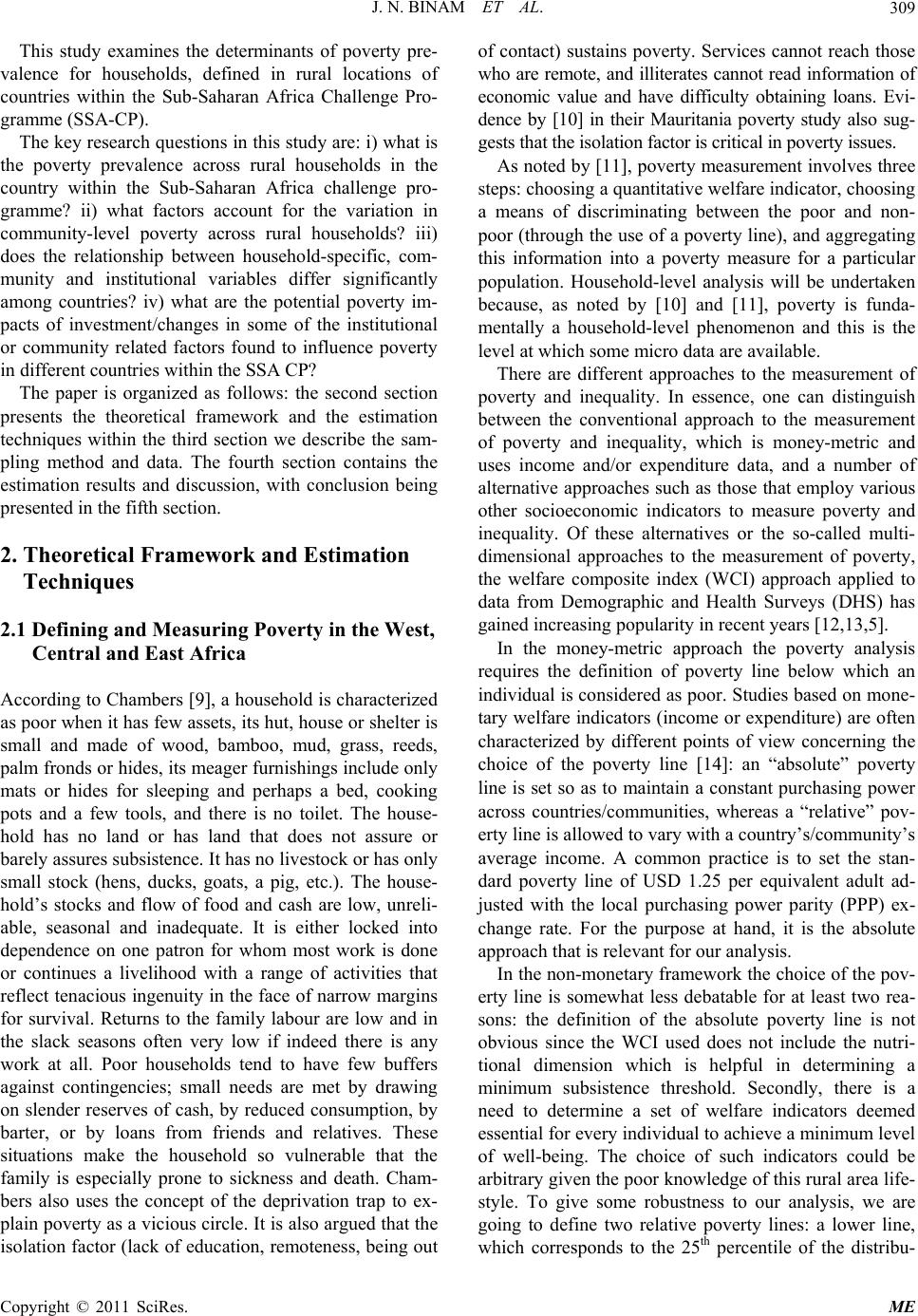

J. N. BINAM ET AL.309
This study examines the determinants of poverty pre-
valence for households, defined in rural locations of
countries within the Sub-Saharan Africa Challenge Pro-
gramme (SSA-CP).
The key research questions in this study are: i) what is
the poverty prevalence across rural households in the
country within the Sub-Saharan Africa challenge pro-
gramme? ii) what factors account for the variation in
community-level poverty across rural households? iii)
does the relationship between household-specific, com-
munity and institutional variables differ significantly
among countries? iv) what are the potential poverty im-
pacts of investment/changes in some of the institutional
or community related factors found to influence poverty
in different countries within the SSA CP?
The paper is organized as follows: the second section
presents the theoretical framework and the estimation
techniques within the third section we describe the sam-
pling method and data. The fourth section contains the
estimation results and discussion, with conclusion being
presented in the fifth section.
2. Theoretical Framework and Estimation
Techniques
2.1 Defining and Measuring Poverty in the West,
Central and East Africa
According to Chambers [9], a household is characterized
as poor when it has few assets, its hut, house or shelter is
small and made of wood, bamboo, mud, grass, reeds,
palm fronds or hides, its meager furnishings include only
mats or hides for sleeping and perhaps a bed, cooking
pots and a few tools, and there is no toilet. The house-
hold has no land or has land that does not assure or
barely assures subsistence. It has no livestock or has only
small stock (hens, ducks, goats, a pig, etc.). The house-
hold’s stocks and flow of food and cash are low, unreli-
able, seasonal and inadequate. It is either locked into
dependence on one patron for whom most work is done
or continues a livelihood with a range of activities that
reflect tenacious ingenuity in the face of narrow margins
for survival. Returns to the family labour are low and in
the slack seasons often very low if indeed there is any
work at all. Poor households tend to have few buffers
against contingencies; small needs are met by drawing
on slender reserves of cash, by reduced consumption, by
barter, or by loans from friends and relatives. These
situations make the household so vulnerable that the
family is especially prone to sickness and death. Cham-
bers also uses the concept of the deprivation trap to ex-
plain poverty as a vicious circle. It is also argued that the
isolation factor (lack of education, remoteness, being out
of contact) sustains poverty. Services cannot reach those
who are remote, and illiterates cannot read information of
economic value and have difficulty obtaining loans. Evi-
dence by [10] in their Mauritania poverty study also sug-
gests that the isolation factor is critical in poverty issues.
As noted by [11], poverty measurement involves three
steps: choosing a quantitative welfare indicator, choosing
a means of discriminating between the poor and non-
poor (through the use of a poverty line), and aggregating
this information into a poverty measure for a particular
population. Household-level analysis will be undertaken
because, as noted by [10] and [11], poverty is funda-
mentally a household-level phenomenon and this is the
level at which some micro data are available.
There are different approaches to the measurement of
poverty and inequality. In essence, one can distinguish
between the conventional approach to the measurement
of poverty and inequality, which is money-metric and
uses income and/or expenditure data, and a number of
alternative approaches such as those that employ various
other socioeconomic indicators to measure poverty and
inequality. Of these alternatives or the so-called multi-
dimensional approaches to the measurement of poverty,
the welfare composite index (WCI) approach applied to
data from Demographic and Health Surveys (DHS) has
gained increasing popularity in recent years [12,13,5].
In the money-metric approach the poverty analysis
requires the definition of poverty line below which an
individual is considered as poor. Studies based on mone-
tary welfare indicators (income or expenditure) are often
characterized by different points of view concerning the
choice of the poverty line [14]: an “absolute” poverty
line is set so as to maintain a constant purchasing power
across countries/communities, whereas a “relative” pov-
erty line is allowed to vary with a country’s/community’s
average income. A common practice is to set the stan-
dard poverty line of USD 1.25 per equivalent adult ad-
justed with the local purchasing power parity (PPP) ex-
change rate. For the purpose at hand, it is the absolute
approach that is relevant for our analysis.
In the non-monetary framework the choice of the pov-
erty line is somewhat less debatable for at least two rea-
sons: the definition of the absolute poverty line is not
obvious since the WCI used does not include the nutri-
tional dimension which is helpful in determining a
minimum subsistence threshold. Secondly, there is a
need to determine a set of welfare indicators deemed
essential for every individual to achieve a minimum level
of well-being. The choice of such indicators could be
arbitrary given the poor knowledge of this rural area life-
style. To give some robustness to our analysis, we are
going to define two relative poverty lines: a lower line,
which corresponds to the 25th percentile of the distribu-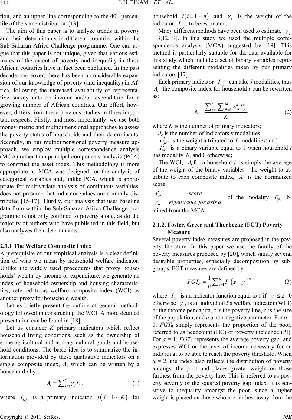

J. N. BINAM ET AL. 310
tion, and an upper line corresponding to the 40th percen-
tile of the same distribution [13].
The aim of this paper is to analyze trends in poverty
and their determinants in different countries within the
Sub-Saharan Africa Challenge programme. One can ar-
gue that this paper is not unique, given that various esti-
mates of the extent of poverty and inequality in these
African countries have in fact been published. In the past
decade, moreover, there has been a considerable expan-
sion of our knowledge of poverty (and inequality) in Af-
rica, following the increased availability of representa-
tive survey data on income and/or expenditure for a
growing number of African countries. Our effort, how-
ever, differs from these previous studies in three impor-
tant respects. Firstly, and most importantly, we use both
money-metric and multidimensional approaches to assess
the poverty status of households and their determinants.
Secondly, in our multidimensional poverty measure ap-
proach, we employ multiple correspondence analysis
(MCA) rather than principal components analysis (PCA)
to construct the asset index. This methodology is more
appropriate as MCA was designed for the analysis of
categorical variables and, unlike PCA, which is appro-
priate for multivariate analysis of continuous variables,
does not presume that indicator values are normally dis-
tributed [15-17]. Thirdly, our analysis that uses baseline
data from within the Sub-Saharan Africa Challenge pro-
gramme is not only confined to poverty alone, as do the
majority of authors who have published in this field, but
also analyzes their determinants.
2.1.1 The Welfare Composite Index
A prerequisite of our empirical analysis is a clear defini-
tion of what we mean by household welfare indicator.
Unlike the widely used procedures that proxy house-
holds’ wealth by income or expenditure, we generate an
index of household ownership and housing characteris-
tics, referred to as welfare composite index (WCI) as
another proxy for household wealth.
Let us briefly present the outline of general method-
ology followed in constructing the WCI. A more detailed
presentation can be found in [18].
Let us consider K primary indicators which reflect
household living conditions, such as the ownership of
some agricultural and non-agricultural goods and house-
hold conditions. The basic idea is to summarize the in-
formation provided by these qualitative indicators on a
single composite index, A, which can be written by a
household i by:
,
1
K
i
jjij
A
I 

 (1)
where is a primary indicator for
household
,ij
I

1jj K


1ii n and
j

is the weight of the
indicator , to be estimated.
,ij
Many different methods have been used to estimate
I
j

[13,12,19]. In this study we used the multiple corre-
spondence analysis (MCA) suggested by [19]. This
method is particularly suitable for the data available for
this study which include a set of binary variables repre-
senting the different modalities taken by our primary
indicators [17].
Each primary indicator ,ij
I
can take J modalities, thus
i
A
the composite index for household i can be rewritten
as:
11
KKJkk
j
kijk
wI
kj
k
i
A
K

 (2)
where K is the number of primary indicators;
Jk is the number of indicators k modalities;
k
j
k
w
k
ijk
is the weight attributed to Jk modalities; and
I
is a binary variable equal to 1 when household i
has modality Jk, and 0 otherwise;
The WCI, i
A
for a household i, is simply the average
of the weight of the binary variables the weight to at-
tribute to each composite index, i
A
is the normalized
score
k
jk
wscore
n value for axeigis a


e of the modality k
ijk
I
b-
tained from the MCA.
2.1.2. Foster, Greer and Thorbecke (FGT) Poverty
Measure
Several poverty index measures are proposed in the pov-
erty literature. In this paper we use the family of the
poverty measures proposed by [20], which satisfy several
desirable properties, especially decomposition by sub-
groups. FGT measures are defined by:

1
1K
yi
j
F
GT y
nI z




 (3)
where
y
I is an indicator function equal to 1 if i yz

0
otherwise i, is an individual i’s welfare indicator (WCI)
or the income per capita, z is the poverty line, n is the size
of the population, and α a non-negative parameter. For α =
0, FGT0 simply represents the proportion of the poor,
referred to as headcount (HC) or poverty incidence (PI).
For α = 1, FGT1 represents the average poverty gap, and
expresses WCI or the level of income necessary for an
individual to be able to reach the poverty threshold. When
α = 2, the index also reflects the distribution of poverty
amongst the poor and places greater weight on those
furthest from the poverty line. This is referred to as pov-
erty severity or the squared poverty gap index. It is sen-
sitive to inequality amongst the poor, since a higher
weight is placed on those who are farthest away from the
y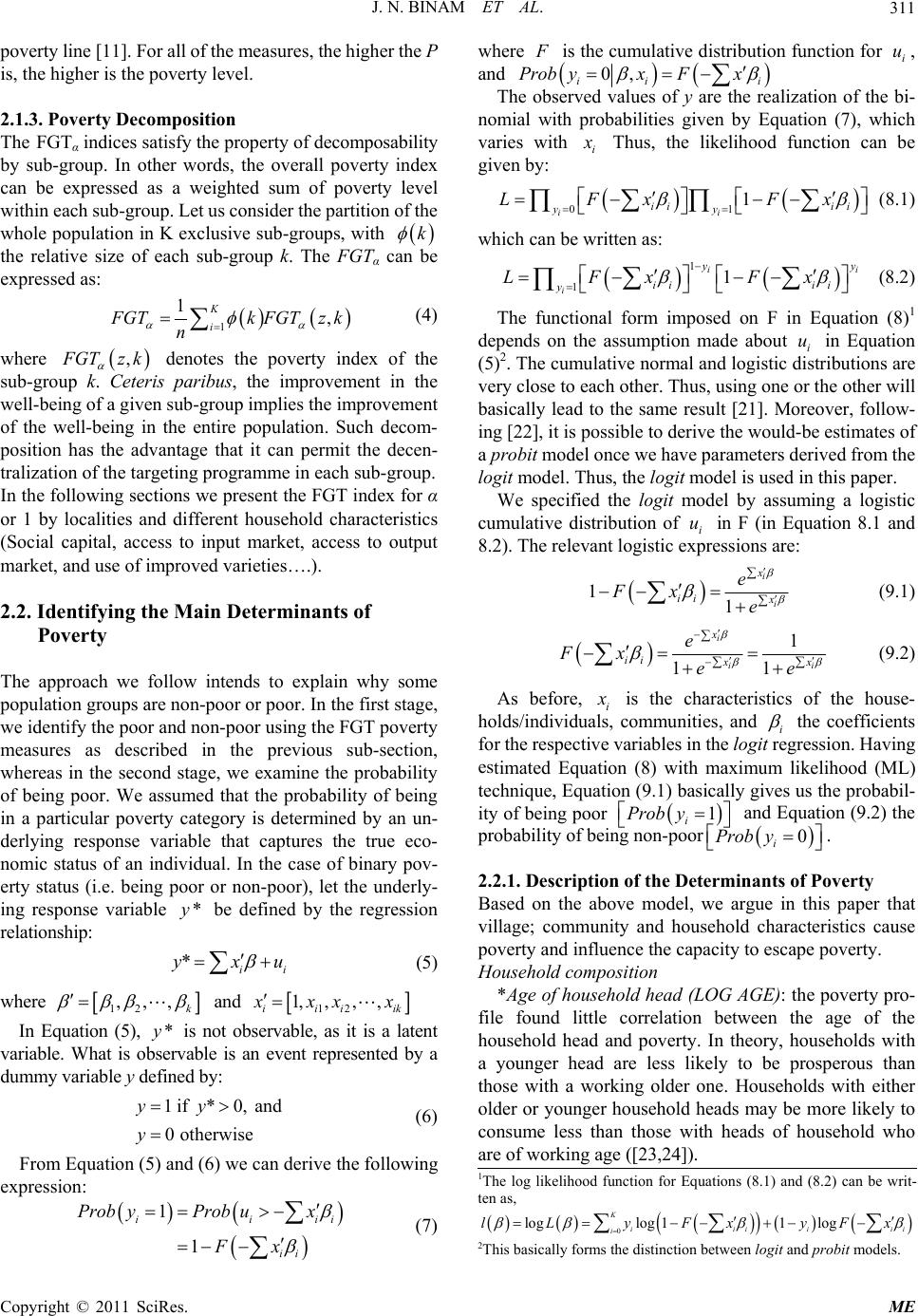

J. N. BINAM ET AL.311
poverty line [11]. For all of the measures, the higher the P
is, the higher is the poverty level.
2.1.3. Po verty Decomposition
The FGTα indices satisfy the property of decomposability
by sub-group. In other words, the overall poverty index
can be expressed as a weighted sum of poverty level
within each sub-group. Let us consider the partition of the
whole population in K exclusive sub-groups, with


k 
the relative size of each sub-group k. The FGTα can be
expressed as:
 
1
1,
K
i
F
GTk FGTz k
n



 (4)
where

,
F
GTz k

denotes the poverty index of the
sub-group k. Ceteris paribus, the improvement in the
well-being of a given sub-group implies the improvement
of the well-being in the entire population. Such decom-
position has the advantage that it can permit the decen-
tralization of the targeting programme in each sub-group.
In the following sections we present the FGT index for α
or 1 by localities and different household characteristics
(Social capital, access to input market, access to output
market, and use of improved varieties….).
2.2. Identifying the Main Determinants of
Poverty
The approach we follow intends to explain why some
population groups are non-poor or poor. In the first stage,
we identify the poor and non-poor using the FGT poverty
measures as described in the previous sub-section,
whereas in the second stage, we examine the probability
of being poor. We assumed that the probability of being
in a particular poverty category is determined by an un-
derlying response variable that captures the true eco-
nomic status of an individual. In the case of binary pov-
erty status (i.e. being poor or non-poor), let the underly-
ing response variable be defined by the regression
relationship:
*y
*ii yxu



 (5)
where


12
,,,
k

 
 and


12
1,,, ,
iiiik
x
xx x

In Equation (5), *
y
is not observable, as it is a latent
variable. What is observable is an event represented by a
dummy variable y defined by:
1 if *0, andyy
0 otherwise y (6)
From Equation (5) and (6) we can derive the following
expression:




1
1
iiii
ii
ProbyProb ux
Fx



 

 

 (7)
F
tion for i u, where is the cumulative distribution func
and

 
0,
ii

i
yx FxProb




d values of y are the realization of the
ic
s with
The observebi-
nomial with probabilities given by Equation (7), whh
varie i
x
Thus, the likelihood function can be
given by:




01
1
ii
ii ii
yy
LFx Fx




   

 

  (8.1)
which can be written as:
 
1
11
ii
i
y
y
ii ii
y
LFx Fx 



 
 

 
  (8.2)
The functional form imposed on F in Equation (8)1
depends on the assumption made about in E
(5)2. The cumulative normal and logistic distributions ar
ve
re
i
uquation
e
ry close to each other. Thus, using one or the other will
basically lead to the same result [21]. Moover, follow-
ing [22], it is possible to derive the would-be estimates of
a probit model once we have parameters derived from the
logit model. Thus, the logit model is used in this paper.
We specified the logit model by assuming a logistic
cumulative distribution of i
u in F (in Equation 8.1 and
8.2). The relevant logistic expressions are:

11
i
i
x
ii x
e
Fx e







  

 (9.1)

1
11
i
ii
x
x
ii x
e
Fx ee





(9.2) 







 


ore, As befi
x
is the characteristics of the house-
holds/individuommunities, and als, ci

the
for the respectie variables in the logit ression. Having
es
coefficients
v reg
timated Equation (8) with maximum likelihood (ML)
technique, Equation (9.1) basically gives us the probabil-
ity of being poor


1
i
Prob y




 and Equation (9.2) the
probability of being non-poor

0
i
Prob y



.
2.2.1. Descriptioninants of Poverty
Based on the above model, we
of the Determ
argue in this paper that
village; community and household characteristics cause
the
erty. In theory, households with
a
poverty and influence the capacity to escape poverty.
Household composition
*Age of household head (LOG AGE): the poverty pro-
file found little correlation between the age of
household head and pov
younger head are less likely to be prosperous than
those with a working older one. Households with either
older or younger household heads may be more likely to
consume less than those with heads of household who
are of working age ([23,24]).
1The log likelihood function for Equations (8.1) and (8.2) can be writ-
ten as,
 






0
loglog 11log
K
iiii
i
lLyFx yFx
ii



 



2This basically forms the distinction between logit and probit models.

J. N. BINAM ET AL. 312
been found in Sierra
Le
d’Ivoire, [28] found household education lev
to
,
re
(a dummy variable = 1 if the household
ons and 0 otherwise)
sehold welfare. The
va
cant variable in a
nu
ing a dummy variable that
age;
e and;
the village resources describing
e
eq
The data used are based on the 2008 baseline survey car-
ithin the Sub-Saharan Africa Challenge pro-
gramme’s pilot learning sites (SSA-CP PLSs). These
LK and ZMM PLSs) of the
SS
*Household size (LOG HHSIZE2): the majority of
studies have found that a larger household size is corre-
lated with increased poverty. It has
one that, poorer households tend to be slighted larger
than non-poor households [24,25] highlight the need to
examine this issue more thoroughly. [26,27], and [28]
used the square of household size as an explanatory
variable to allow for non-linearity in the relationship
between household size and living standards. Other
things being equal, we expect smaller households to be
less poor and, following other research, the square of
household size is included as an independent variable. In
addition, households with a higher share of children are
likely to have fewer income-generating opportunities
than those with more adults of working age. The regres-
sions include variables for the proportion of children
below the age of 16 in the household (CHILDRAT) and
that of adults between the ages of 16 and 59 (ADUL-
TRAT).
*Education: the poverty profile showed many correla-
tions between education levels and poverty. In examin-
ing Côteels  -RESPOND6 a dummy variable indicating if there is
any agro-dealer shop within the community/village.
*Variables related to
be a key determinant of poverty in urban, but not in
rural areas. [27] found that education, specifically
women’s education, was a key determinant of household
poverty status. Similarly, [26] (2003) found that higher
levels of education in Malawi resulted in welfare im-
provements. [29], on the other hand, using a different
data set for Mozambique, found that education was not a
significant factor in poverty levels, especially for rural
households. The education variables used in this analysis
included the level of education of the household head
(POSTSEC and POSTPEDU being a dummy variables =
1 if the household head attained post secondary or post
primary education respectively and 0 otherwise).
*Social capital: [30] found that higher levels of social
capital, as measured by involvement in associations to
reflect social norms and relationships in a community
sult in higher levels of welfare. [29] also found this to
be the case in Mozambique. To capture possible effects
of community involvement, a dummy variable for
whether or not someone in the household participates in
community programmes is included. These variables are
specified as:
 MEMBERSHIP (a dummy = 1 if the household head
or any other member belong to a community group);
 EXPEXTN
had contact with agricultural extension agents and 0
otherwise)
 RESEARCH (a dummy variable = 1 indicating if the
household participated in the community research
demonstrati
*Remittances: This is the only variable for income
source used, but if it can be considered an extra source of
income, it is likely to improve hou
riable is a simple dummy variable for whether or not
the household receives remittances.
Access to infrastructure: Given that poverty was sig-
nificantly higher in rural areas, access to infrastructure
has also been found to be a signifi
mber of other studies. [28] found that, in rural areas,
infrastructure has substantial predictive power: house-
holds located in villages that are nearer to paved roads
and public markets are better-off. A series of dummy
variables have been included in the model to pick up
localized effects. These are:
*Variables related to input and output market access
including:
 -Variable RESPOND1 be
indicates if there is any market within the commu-
nity/vill
 -Variable RESPOND3 a dummy indicating if there is
any trader or processor being linked with the com-
munity/villag
the possession of some physical amenities in the com-
munity/village. These are dummy variables defined to b
ual to one each if the village/community is endowed
with the following: schools (POSSES1), hospital, clinic
or other health center (POSSES2), worship places
(POSSES3), social halls or centers (POSSES4), boreholes
or wells (POSSES5), cattle dips, veterinary centers (POS-
SES6), radio-reception channels (POSSES9), all weather
roads (POSSES11), livestock watering points (POS-
SES14), rural micro-finance bank (POSSES16), govern-
ment extension agriculture/livestock office (POSSES17)
and, agricultural research site (POSSES18).
3. Data
ried out w
data were collected for the seven countries and covered
nearly five thousand households. The fundamental ra-
tionale behind the choice of a household as a unit of
analysis is the assumption of sharing of resources among
households.
The data gathered as part of the Kano, Katsina, Maradi,
Lake Kivu and Zimbabwe, Malawi and Mozambique
pilot learning site (KKM,
A CP provide rich information at the individ-
ual/farmer, the household, the village and the community
level. The data include information on the awareness and

J. N. BINAM ET AL.313
um number
ap
possession of agricultural equipment, ownership of
du
th
4.1. Poverty Analysis Results
The choice of poverty line is crucial for poverty analysis
apparent non-arbitrary
level at which to set it. The poverty lines set by [13] were,
ion of an absolute poverty line is
no
in
adoption of improved crop varieties, food production,
access to inputs, capital assets, social capital, house-
hold/farmer characteristics, market and marketing, house-
hold income and expenditure, food security/insecurity,
dietary, credit, agricultural practices and knowledge,
amongst others. Table 1 below provides the distribution
of households by country, sub-countries and villages,
while Table 2 gives the descriptive statistics of variables
used to identify the determinants of poverty.
As shown in Table 2, the number of households with
members belonging to a farmer group or organization
varies from 10% to 51% with the maxim
pearing in Uganda (51%). Throughout the countries,
on average, less than 20% of the households have had
contact with agricultural extension agents or participated
in community research demonstrations. Moreover, very
few communities in these countries possess cattle dips,
veterinary centers, all weather roads livestock watering
points, rural micro-finance bank, government extension
agriculture/livestock office and, agricultural research
site.
To construct the wealth index, we select fourteen pri-
mary indicators that can be classified into three catego-
ries:
rable goods and housing conditions. Table 3 presents
a detailed description of these indicators. [19] describes
the calculation of a composite poverty indicator using
MCA as a four-stage process. Firstly, one constructs an
indicator matrix (of ones and zeros) that shows the asset
ownership of each household. If the households are dis-
played as rows, each asset is represented by the inclusion
of a column for each possible (mutually exclusive and
exhaustive) ownership category of that asset. In other
words, each categorical asset ownership variable is re-
duced to a set of binary indicators. In this way, every
household will indicate a ‘‘1’’ in exactly one of each
asset’s set of columns or categories, and a ‘‘0’’ in all
other columns. Secondly, the profiles of the households
relative to the categories of asset ownership are calcu-
lated. The row profiles of a matrix are the rows of that
matrix, each divided by its row sum. Thirdly, MCA is
applied to the original indicator matrix, and provides a
set of category-weights from the first dimension or fac-
torial axis of the analysis results. Fourthly, these MCA
category-weights are applied to the profile matrix. A
household’s MCA composite indicator score is calcu-
lated by adding up all of that unit’s weighted responses.
The Table 3, which also reports the weights for each
index component, shows that those components that re-
flect higher standards of living contribute positively to
e asset index, while components that reflect lower
standards of living contribute negatively to the wealth
index across countries. For example, owning a bicycle,
owing a draft cattle or having a house with a good qual-
ity roofing material increases a household’s asset index
score in some countries; while not owning a bicycle, a
radio, or living in a house with poor floor quality de-
creases a household’s asset index score, that is, measured
level of welfare.
4. Results
using FGT measures. There is no
compared to their earlier study [13], set at relatively high
levels, where the discrimination ability of asset indices
was somewhat better.
In our non-monetary poverty framework the choice of
the poverty line is somewhat less debatable for two rea-
sons. Firstly, the definit
t obvious since the welfare composite index used here
does not include the nutritional dimension which is
helpful in determining a minimal subsistence threshold.
Secondly, there is a need to determine a set of welfare
indicators deemed essential for every individual to
achieve a minimum level of well-being. Based on this
second reason, we chose one higher poverty line set at
the 75th percentile because Africa has substantially
higher level of poverty than other world regions and the
asset index does not discriminate well at very low levels.
Table 4 presents the monetary-based poverty indicators
of households estimated using the standard poverty line
of USD 1.25 per equivalent adult adjusted with the local
purchasing power parity (PPP) exchange rate, below
which a household was classified as being poor and
above which a household was classified as being
non-poor, while Table 5 provides a summary of the
monetary and non-monetary-based poverty indicators.
The poverty measures include the headcount index, the
poverty gap, and the squared poverty gap. The headcount
index is the percentage of the population living
households with income per capita below the poverty
threshold. However, the headcount index ignores the
amounts by which the income of the poor falls short of
the poverty threshold. Hence the poverty gap index
which gives the mean distance below the poverty line as
a proportion of the poverty line is also computed, the
squared poverty gap index which indicates the severity
of poverty is computed by weighting the individual pov-
erty gaps by the gaps themselves, so as to reflect ine-
quality among the poor.
From the summary in Table 5, it is clear that commu-
nities in the study area deal with pervasive rural poverty: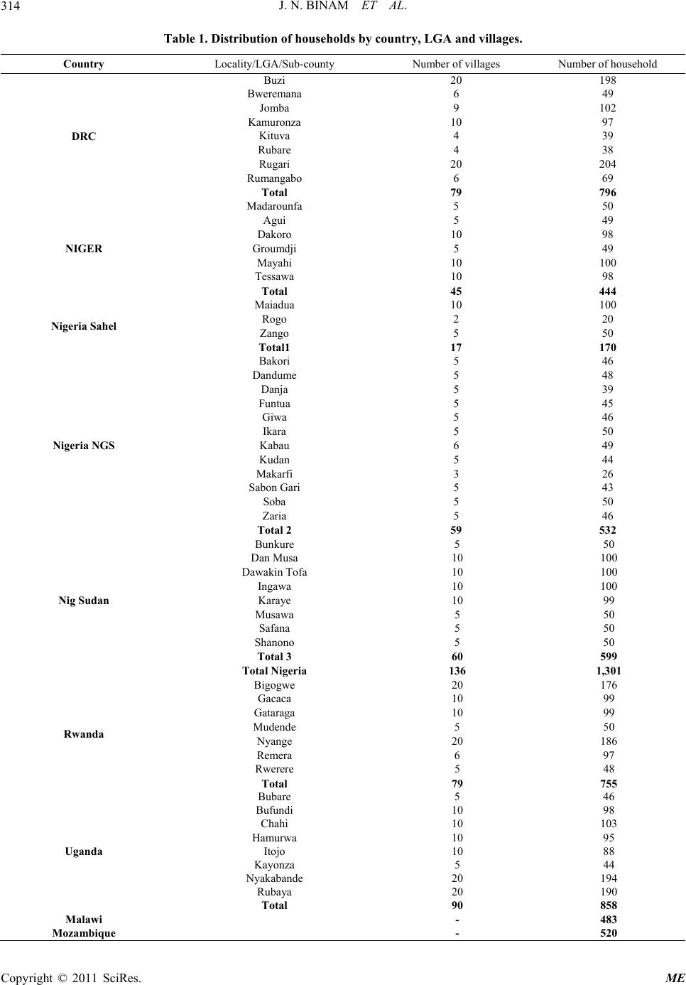

J. N. BINAM ET AL. 314
Table 1. Distribution of households
Number of household
bycountry, LGA and villages.
Country Locality/LGA/Sub-county Number of villages
Buzi 20 198
Bweremana 6 49
Jomba 9 102
Kamuronza 10 97
Kituva 4 39
Rubare 4 38
Rugari 20 204
Ro
DRC
NIGER
Nigeria Sahel
D
Sabon Gari
Nigeria NGS
B
D
D
Nig Sudan
Toa 1,
Rwanda
N
Uganda
Malawi
Mozambique
umangab6 69
Total 79 796
Madarounfa 5 50
Agui 5 49
Dakoro
Gri
10 98
oumdj5 49
Mayahi 10 100
Tessawa 10 98
Total 45 444
Maiadua 10 100
Rogo 2 20
Zango 5 50
Total1 17 170
Bakori 5 46
andume 5 48
Danja 5 39
Funtua 5 45
Giwa 5 46
Ikara 5 50
Kabau 6 49
Kudan 5 44
Makarfi 3 26
5 43
Soba 5 50
Zaria
T5 46 otal 2 59 532
unkure 5 50
an Musa 10 100
awakin Tofa 10 100
Ingawa 10 100
Karaye 10 99
Musawa 5 50
Safana 5 50
Shanono 5 50
Total 3 60 599
tal Nigeri136 301
Bigogwe 20 176
Gacaca 10 99
Gataraga 10 99
Mudende 5 50
Nyange 20 186
Remera 6 97
Rwerere 5 48
Total 79 755
Bubare
B
5 46
ufundi 10 98
1 Chahi 1003
Hamurwa 10 95
Itojo 10 88
Kayonza
ya de
5 44
kaban20 194
Rubaya 20190
Total 90 858
-
-
483
520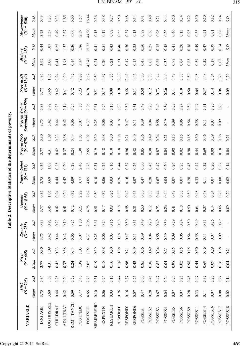

J. N. BINAM ET AL.315
Table 2. Descriptive Statistics of the determinants of poverty.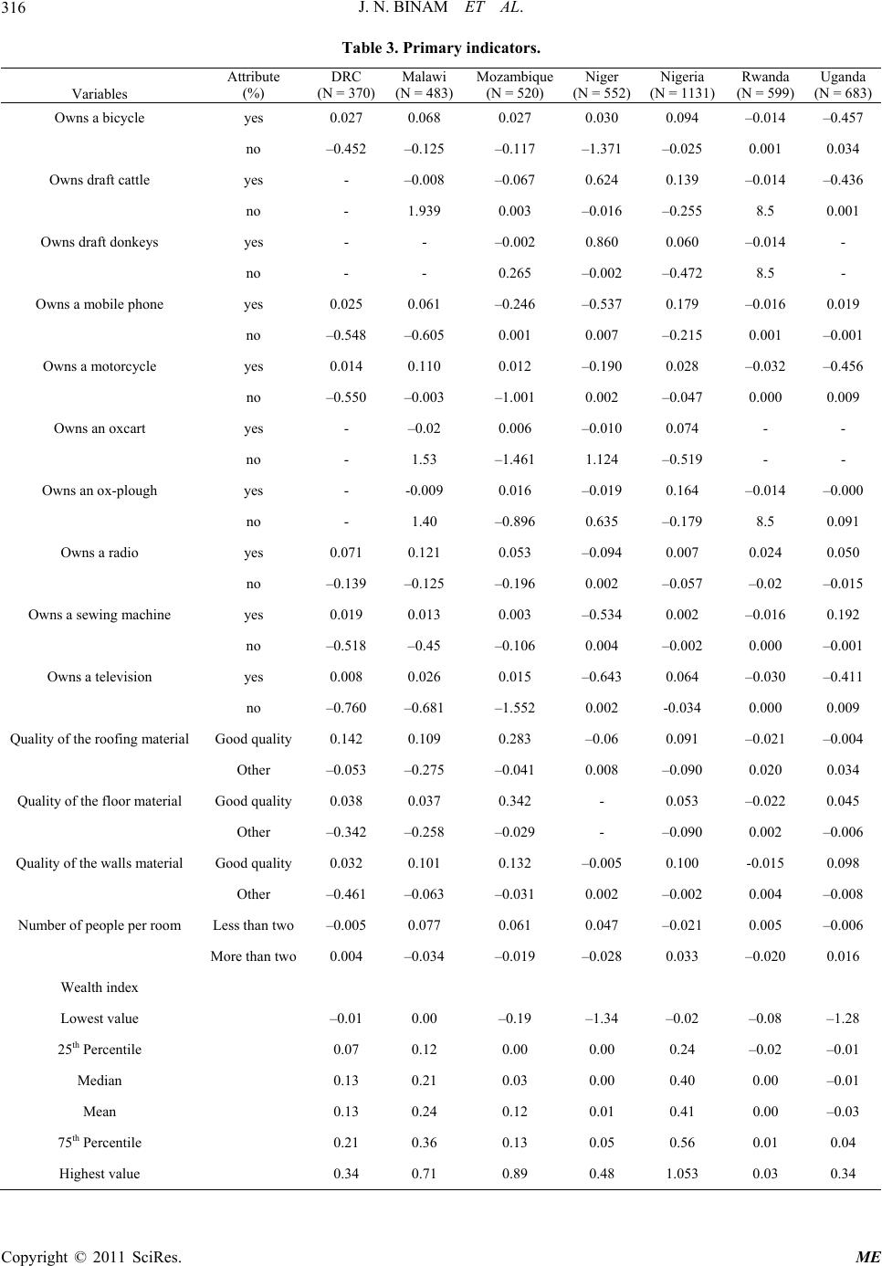

J. N. BINAM ET AL. 316
Table 3. Primary indicators.
Variables
Attribute
(%)
DRC
(N = 370)
Malawi
(N = 483)
Mozambique
(N = 520)
Niger
(N = 552)
Nigeria
(N = 1131)
Rwanda
(N = 599)
Uganda
(N = 683)
Owns a bicycle yes 0.027 0.068 0.027 0.030 0.094 –0.014 –0.457
no –0.452 –0.125 –0.117 –1.371 –0.025 0.001 0.034
Owns draft cattle yes - –0.008 –0.067 0.624 0.139 –0.014 –0.436
no - 1.939 0.003 –0.016 –0.255 8.5 0.001
Owns draft donkeys yes - - –0.002 0.860 0.060 –0.014 -
no - - 0.265 –0.002 –0.472 8.5 -
Owns a mobile phone yes 0.025 0.061 –0.246 –0.537 0.179 –0.016 0.019
no –0.548 –0.605 0.001 0.007 –0.215 0.001 –0.001
Owns a motorcycle yes 0.014 0.110 0.012 –0.190 0.028 –0.032 –0.456
no –0.550 –0.003 –1.001 0.002 –0.047 0.000 0.009
Owns an oxcart yes - –0.02 0.006 –0.010 0.074 - -
no - 1.53 –1.461 1.124 –0.519 - -
plough yes - -0.009 0.016 –0.019 0.164 –0.014 –0.000
no - 1.40 –0.896 0.635 –0.179 8.5 0.091
Owns a radio yes 0.071 0.121 0.053 –0.094 0.007 0.024 0.050
no –0.139 –0.125 –0.196 0.002 –0.057 –0.02 –0.015
ns a sewing machine yes 0.019 0.013 0.003 –0.534 0.002 –0.016 0.192
no –0.518 –0.45 –0.106 0.004 –0.002 0.000 –0.001
yes 0.008 0.026 0.015 –0.643 0.064 –0.030 –0.411
no –0.760 –0.681 –1.552 0.002 -0.034 0.000 0.009
Quality of the roofing material Good quality 0.142 0.109 0.283 –0.06 0.091 –0.021 –0.004
Other –0.053 –0.275 –0.041 0.008 –0.090 0.020 0.034
of the floor material Good quality 0.038 0.037 0.342 - 0.053 –0.022 0.045
Other –0.342 –0.258 –0.029 - –0.090 0.002 –0.006
Quality of the walls material Good quality 0.032 0.101 0.132 –0.005 0.100 -0.015 0.098
Other –0.461 –0.063 –0.031 0.002 –0.002 0.004 –0.008
Number of people per room Less than two –0.005 0.077 0.061 0.047 –0.021 0.005 –0.006
More than two 0.004 –0.034 –0.019 –0.028 0.033 –0.020 0.016
Wealth index
Lowest value –0.01 0.00 –0.19 –1.34 –0.02 –0.08 –1.28
25th Percentile 0.07 0.12 0.00 0.00 0.24 –0.02 –0.01
Median 0.13 0.21 0.03 0.00 0.40 0.00 –0.01
Mean 0.13 0.24 0.12 0.01 0.41 0.00 –0.03
75th Percentile 0.21 0.36 0.13 0.05 0.56 0.01 0.04
Highest value 0.34 0.71 0.89 0.48 1.053 0.03 0.34
Owns an ox-
Ow
Owns a television
Quality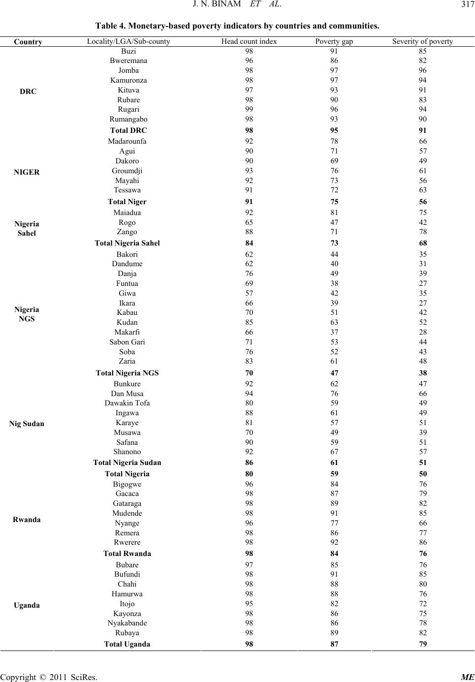

J. N. BINAM ET AL.317
Table 4. Monetary-basries and communities.
Country Locality/Lunty unS ov
ed poverty indicators by count
GA/Sub-coHead cot index Poverty gap everity of perty
Bu8 zi 991 85
Bwere 96
Jom
Kamua 98
Kituva 97
Rub98
Rug99
Rumangabo 98 90
DRC
Total DRC 98
Madarounfa 92 66
Ag90
Dak90
Groum
May92
Tessawa 91
NIGER
Total Niger 91
Maiadua 92
Rogo 65 47 42
Zan88 78
Nigeria
Sa Total Nigeria Sahel 84 68
Bakor35
Dand
Danja 76 39
Fun69
Giw57
Ikar66
Kab70
Kudan 85 63 52
Mak66
Sabon Gari 71
Sob76
Zar83
Nigeria
NGS
Total Nigeria NGS 70 47 38
Bunk92
D94
a80
Ing88
Karaye 81 57 51
70 49
Safana 90 59
Shanono 92 67
Nig Sudan
tal Nigeria Sudan 86
Total Nigeria 80 59 50
Bigogwe 96
98
98
98
Nyange 96 77 66
Reme86 77
Rwerere 98
Rwanda
Total Rwanda 98
Bubar5
Bufundi 98 91 85
Chah98 8 0
Hamurwa 98 8 6
Itojo 95 2 2
Kayonza 98 6 5
Nyakabande 98
Rubay 2
Uganda
Total Uganda 98 87 79
mana
ba 98
86
97
82
96
ronz97 94
93
90
91
83are
ari 96
93
94
9591
78
71ui 57
oro
dji 93
69
76
49
61
ahi 7356
72
75
63
56
81 75
go 71
hel 73
44 i 62
ume 62 4031
49
38tua 27
a
a
42
39
35
27
au 5142
arfi 3728
53
52
44
43a
ia 6148
ure 6247
an Musa
wakin Tofa
76
59
66
49 D
awa 6149
Musawa 39
51
57
To 61 51
84 76
Gacaca
Gataraga
87
89
79
82
Mudende 9185
ra 98
92
84
86
76
e 97 876
i 88
8
8
7
7
8 7
86
89
78
8a 98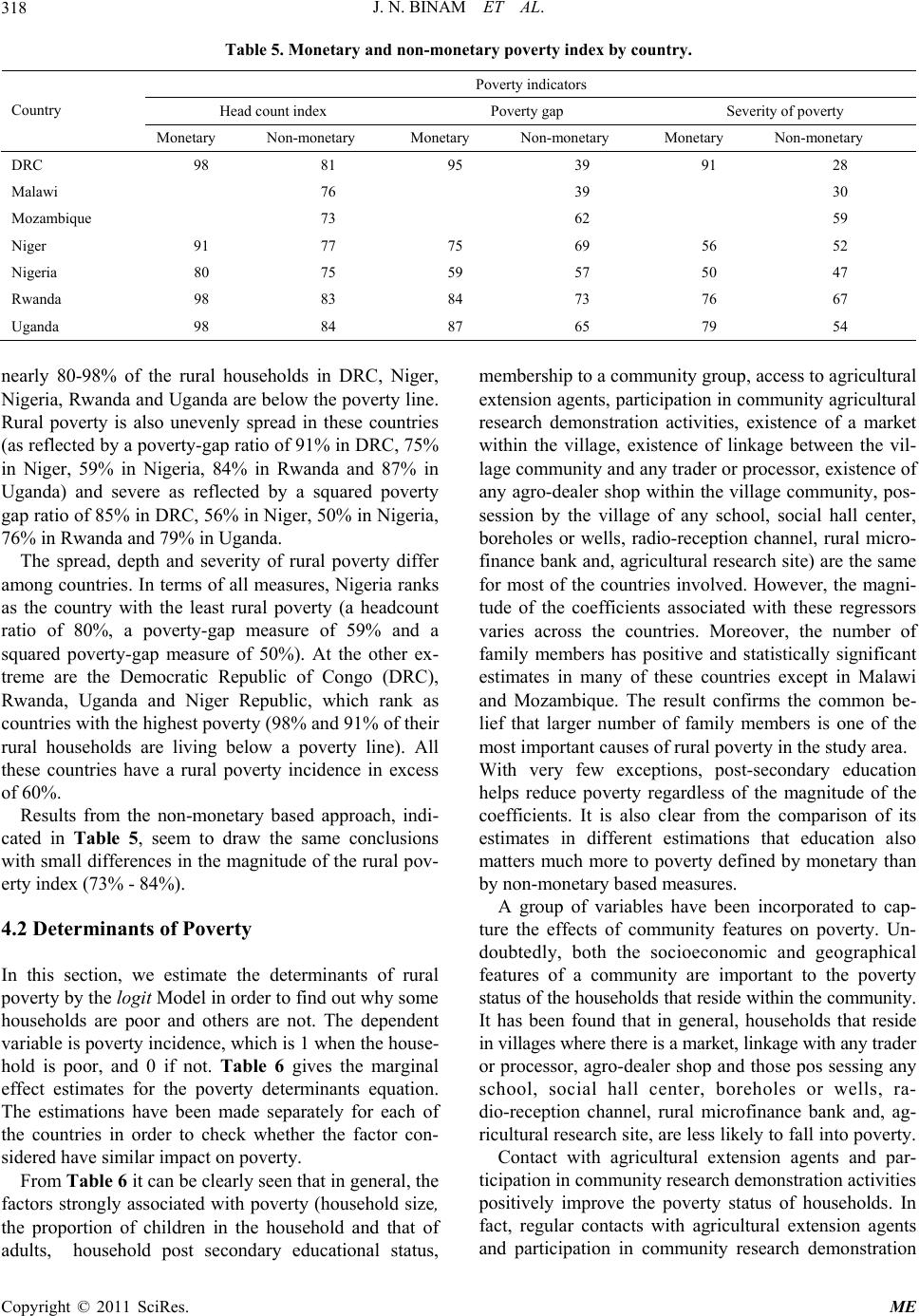

J. N. BINAM ET AL. 318
icators
Table 5. Monetary and non-monetary pove rty index by country.
Poverty ind
Head count index ty gap Severity of pty Poverover
Country
Monetary Non-monetary Monetary Non-monetary Monetary Non-etary mon
DRC 98 81 95 39 91 28
Malawi 76 39 30
Mozambique 73 62 59
Niger 91 77 75 69 56 52
Nigeria 80 75 59 57 50 47
Rwanda 98 83 84 73 76 67
Uganda 98 84 87 65 79 54
nearly 80-98% of the ruran DRC, Niger,
Nigeria, Rwanda and Uganw the poverty line.
Rurty is also unevenad in these countries
(as d by a poverty-gapof 91% in DRC, 75%
in Niger, 59% in Nigeda and 87% in
Uganda) and severe as refly a squared poverty
gap ratio of 85% in DRC, 5er, 50% in Nigeria,
76% in Rwanda and 79% in .
The spread, depth and sevf rural poverty differ
amongntries. In terms of easures, Nigeria ranks
as the country with the leastpoverty (a headcount
ratio o80%, a poverty-gasure of 59% and a
squared poverty-gap meas). At the other ex-
treme are the Democratic Rlic of Congo (DRC),
Rwanda, Uganda and Nigerblic, which rank as
countries with the highend 91% of their
rural households are livinga poverty line). All
these countries have a rucidence in excess
of 60%.
om the non-monased approach, indi-
cated in Table 5, seem to e same conclusions
with small differences in theude of the rural pov-
erty index (73% - 84%)
4.2 Determinants of Po
In this section, we estimaterminants of rural
po logit Model find out why some
households are poor and ot not. The dependent
variable is poverty incidence1 when the house-
hold is poor, and 0 if noives the marginal
effect estimates for the povterminants equation.
The estimations have been parately for each of
the countries in order to chther the factor con-
side similar impact .
From ble 6 it can be clearly seen that in general, the
factors strongly associatedty (household size,
the proportion of children iousehold and that of
adults, household post ducational status,
mbership to a com accessgricultural
tension agents, participation in community agricultural
earch demonstration activities, existence of a market
thin the village, existence of linkage between the vil-
e community and trader or processoxistence of
y agro-dealer shop within the village community, pos-
sion by the villagny school, social hall center,
reholes or wells, ro-reception channel, rural micro-
ance bank and, agltural research site) are the same
ost of the countries involved. Howevagni-
e of the coefficients associated with th regressors
ries across the ctries. Moreover, the number of
ily members has positive and statistically significant
imates in many oese countries excin Malawi
d Mozambique. The result confirms the common be-
f that larger numbof family members is one of the
st important causf rural poverty in thtudy area.
ith very few extions, post-seconducation
lps reduce povertygardless of the maude of the
efficients. It is al from the comparison of its
imates in different estimations that education also
tters much more to poverty defined by etary than
non-monetary basmeasures.
A group of variables have been incorped to cap-
e the effects of cmunity features onverty. Un-
ubtedly, both the socioeconomic and geographical
tures of a commty are important te poverty
tus of the households that reside within the community.
has been found thn general, househothat reside
villages where there is a market, linkage with any trader
processor, agro-dealer shop and those pos sessing any
hool, social hall center, boreholes wells, ra-
-reception channel, rural microfinance k and, ag-
ultural research site, are less likely to fato poverty.
Contact with agricultural extension agents and par-
ipation in commun research demonstrn activities
sitively improve tpoverty status of households. In
t, regular contactith agricultural extension agents
d participation inunity research onstration
l
da are belo
households i
ral pove
reflecte
ly spre
ratio
ria, 84% in Rwan
ected b
6% in Nig
Uganda
erity o
cou
f
all m
rural
p mea
ure of 50%
epub
Repu
st poverty (98% a
below
ral poverty in
Results fretary b
draw th
magnit
.
verty
te the de
verty by thein order to
hers are
, which is
t. Table 6 g
erty de
made se
e e
on erty
ck wh
ered hav
Ta pov
with pover
n the h
secondary e
memunity group, to a
ex
res
wi
lag anyr, e
an
sese of a
bo adi
fin ricu
for mer, the m
tud ese
va oun
fam
estf thept
an
lieer
moes oe s
Wcepary ed
he regnit
coso clear
est
ma mon
byed
orat
tur om po
do
feaunio th
sta
It at ilds
in
or
scor
dio ban
ric ll in
tic ity atio
pohe
facs w
an commdem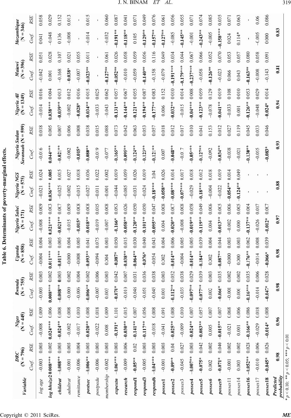

J. N. BINAM ET AL.319
* p < 0.10; ** p < 0.
Table 6. Determinants of poverty-marginal effects.
05; *** p < 0.01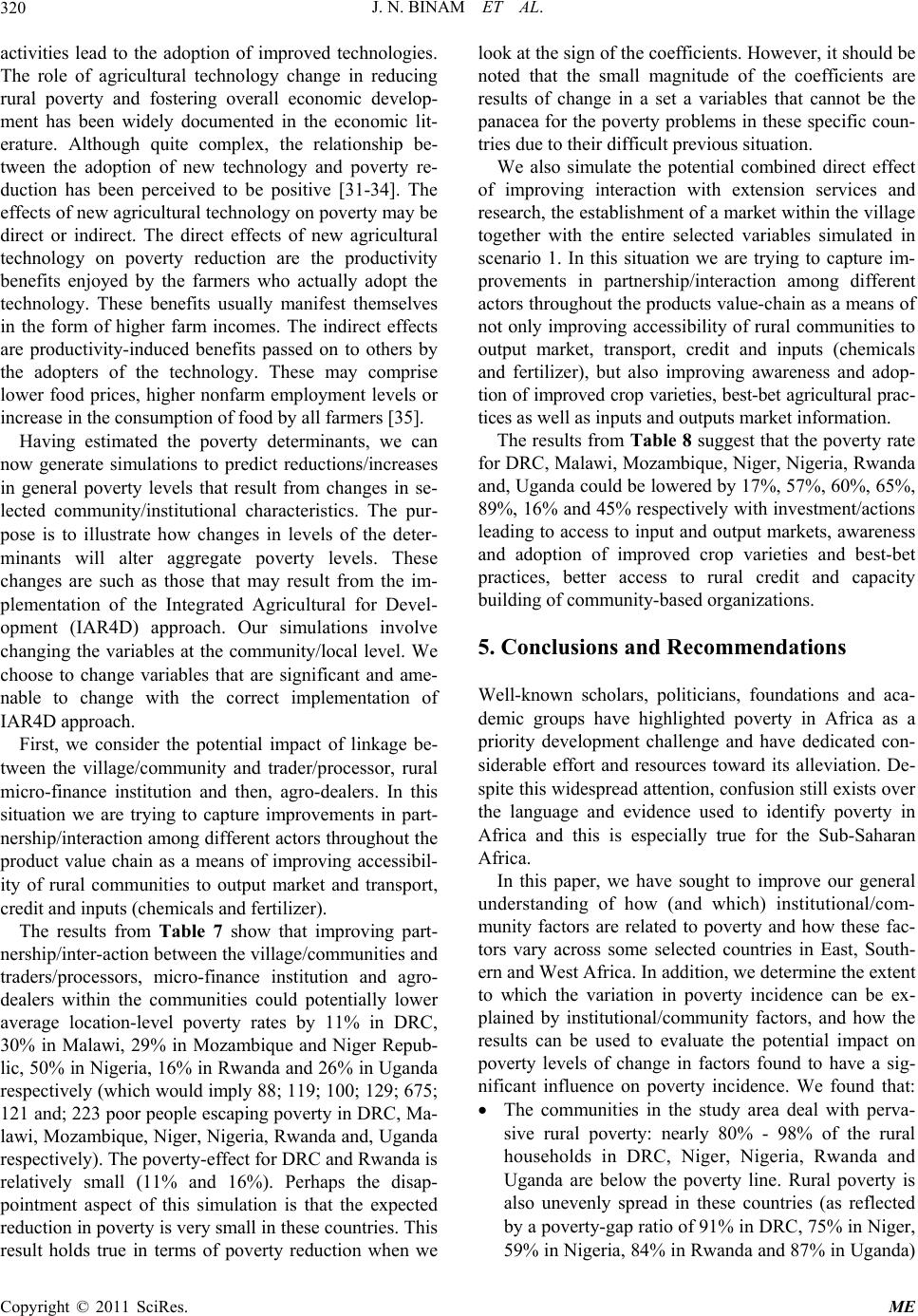

J. N. BINAM ET AL. 320
activities lead to the adoption of improved technologies.
The role of agricultural technology change in reducing
rural poverty and fostering overall economic develop-
ment has been widely documented in the economic lit-
erature. Although quite complex, the relationship be-
tween the adoption of new technology and poverty re-
duction has been perceived to be positive [31-34]. The
effects of new agricultural technology on poverty may be
direct or indirect. The direct effects of new agricultural
technology on poverty reduction are the productivity
benefits enjoyed by the farmers who actually adopt the
technology. These benefits usually manifest themselves
in the form of higher farm incomes. The indirect effects
are productivity-induced benefits passed on to others by
the adopters of the technology. These may comprise
lower food prices, higher nonfarm employment levels or
increase in the consumption of food by all farmers [35].
Having estimated the poverty determinants, we can
now generate simulations to predict reductions/increases
in general poverty levels that result from changes in se-
lected community/institutional characteristics. The pur-
pose is to illustrate how changes in levels of the deter-
minants will alter aggregate poverty levels. These
changes are such as those that may result from the im-
plementation of the Integrated Agricultural for Devel-
opment (IAR4D) approach. Our simulations involve
changing the variables at the community/local level. We
choose to change variables that are significant and ame-
nable to change with the correct implementation of
IAR4D approach.
First, we consider the potential impact of linkage be-
tween the village/community and trader/processor, rural
micro-finance institution and then, agro-dealers. In this
situation we are trying to capture improvements in part-
nership/interaction among different actors throughout the
product value chain as a means of improving accessibil-
ity of rural communities to output market and transport,
credit and inputs (chemicals and fertilizer).
The results from Table 7 show that improving part-
nership/inter-action between the village/communities and
traders/processors, micro-finance institution and agro-
dealers within the communities could potentially lower
average location-level poverty rates by 11% in DRC,
30% in Malawi, 29% in Mozambique and Niger Repub-
lic, 50% in Nigeria, 16% in Rwanda and 26% in Uganda
respectively (which would imply 88; 119; 100; 129; 675;
121 and; 223 poor people escaping poverty in DRC, Ma-
lawi, Mozambique, Niger, Nigeria, Rwanda and, Uganda
respectively). The poverty-effect for DRC and Rwanda is
relatively small (11% and 16%). Perhaps the disap-
pointment aspect of this simulation is that the expected
reduction in poverty is very small in these countries. This
result holds true in terms of poverty reduction when we
look at the sign of the coefficients. However, it should be
noted that the small magnitude of the coefficients are
results of change in a set a variables that cannot be the
panacea for the poverty problems in these specific coun-
tries due to their difficult previous situation.
We also simulate the potential combined direct effect
of improving interaction with extension services and
research, the establishment of a market within the village
together with the entire selected variables simulated in
scenario 1. In this situation we are trying to capture im-
provements in partnership/interaction among different
actors throughout the products value-chain as a means of
not only improving accessibility of rural communities to
output market, transport, credit and inputs (chemicals
and fertilizer), but also improving awareness and adop-
tion of improved crop varieties, best-bet agricultural prac-
tices as well as inputs and outputs market information.
The results from Table 8 suggest that the poverty rate
for DRC, Malawi, Mozambique, Niger, Nigeria, Rwanda
and, Uganda could be lowered by 17%, 57%, 60%, 65%,
89%, 16% and 45% respectively with investment/actions
leading to access to input and output markets, awareness
and adoption of improved crop varieties and best-bet
practices, better access to rural credit and capacity
building of community-based organizations.
5. Conclusions and Recommendations
Well-known scholars, politicians, foundations and aca-
demic groups have highlighted poverty in Africa as a
priority development challenge and have dedicated con-
siderable effort and resources toward its alleviation. De-
spite this widespread attention, confusion still exists over
the language and evidence used to identify poverty in
Africa and this is especially true for the Sub-Saharan
Africa.
In this paper, we have sought to improve our general
understanding of how (and which) institutional/com-
munity factors are related to poverty and how these fac-
tors vary across some selected countries in East, South-
ern and West Africa. In addition, we determine the extent
to which the variation in poverty incidence can be ex-
plained by institutional/community factors, and how the
results can be used to evaluate the potential impact on
poverty levels of change in factors found to have a sig-
nificant influence on poverty incidence. We found that:
 The communities in the study area deal with perva-
sive rural poverty: nearly 80% - 98% of the rural
households in DRC, Niger, Nigeria, Rwanda and
Uganda are below the poverty line. Rural poverty is
also unevenly spread in these countries (as reflected
by a poverty-gap ratio of 91% in DRC, 75% in Niger,
59% in Nigeria, 84% in Rwanda and 87% in Ugana)
d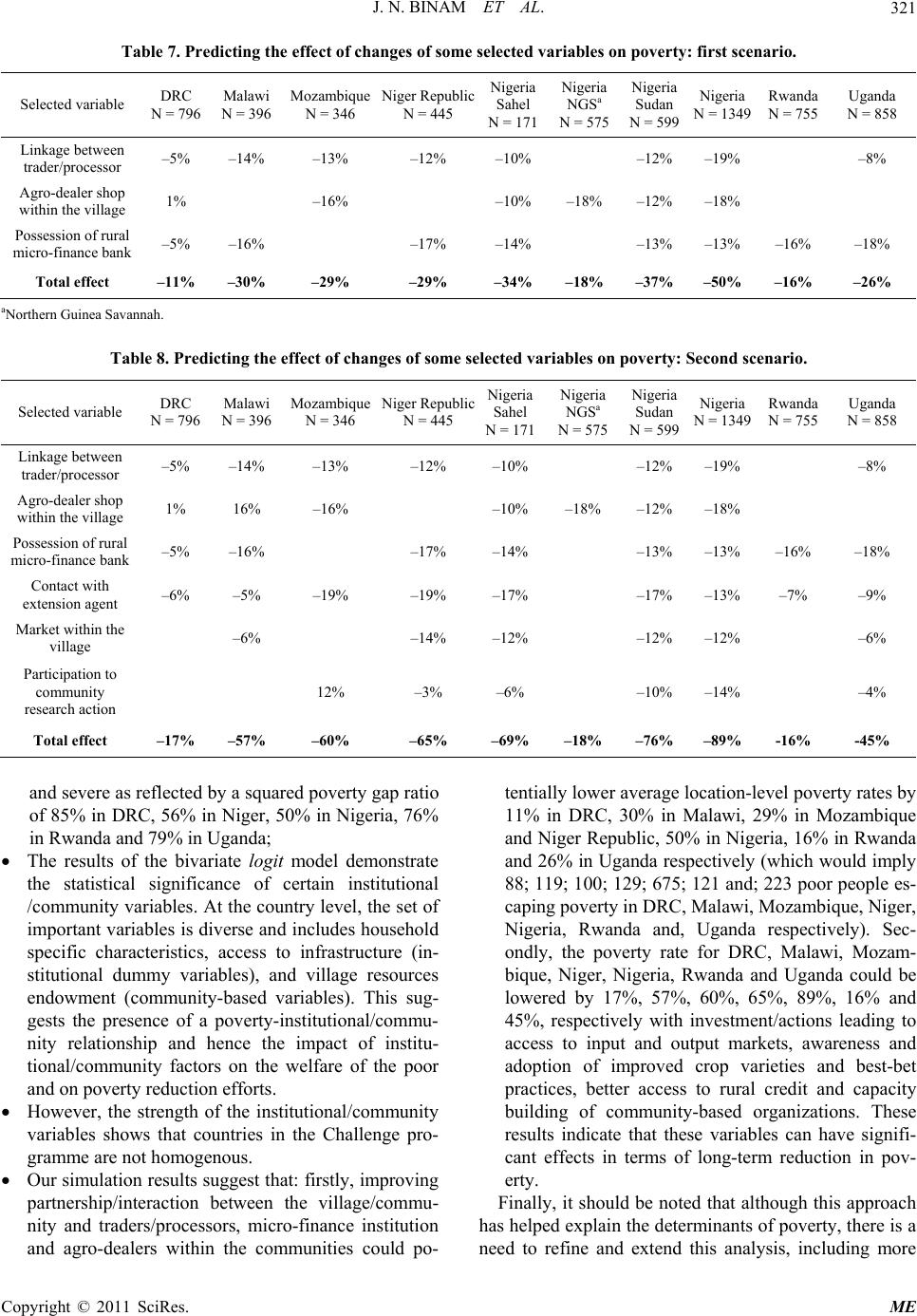

J. N. BINAM ET AL. 321
me
ublic
5
Table 7. Predicting the effect of changes of so
Selected variable DRC
N = 796
Malawi
N = 396
Mozambique
N = 346
Niger Rep
N = 44
selected variables on poverty: first scenario.
Nigeria
Sahel
N = 171
Nigeria
NGSa
N = 575
Nigeria
Sudan
N = 599
Nigeria
N = 1349
Rwanda
N = 755
Uganda
N = 858
Linkage between
trader/processor –5% –14% –13% –12% –10% –12%–19% –8%
Agro-dealer shop
within the village 1% –16%
Possession of rural
micro-finance bank –5% –16% –17%
Total effect –11% –30% –29% –29%
–10% –18% –12%–18%
–14% –13%–13% –16% –18%
–34%–18% –37%–50% –16% –26%
aNorthern Guinea Savannah.
Table 8. Predicting the effect of changes of som
Selected variable DRC
N = 796
Malawi
N = 396
Mozambique
N = 346
Niger Repu
N = 4
e se
blic
45
lected variables on poverty: Second scenario.
Nigeria
Sahel
N
Nigeria
NGSa
Nigeria
Sudan Nigeria
N = 1349
Rwanda
N = 755
Uganda
N = 858
= 171N = 575N = 599
Linkage between
trader/processor –5% –14% –13% –12% –10% –12%–19% –8%
Agro-dealer shop
within the village 1% 16% –16%
Possession of rural
micro-finance bank –5% –16% –17%
Contact with
extension agent –6% –5% –19% –19%
Market within the
village –6% –14%
Participation to
community
research action
12% –3%
–10% –18% –12%–18%
–14% –13%–13% –16% –18%
–17% –17%–13% –7% –9%
–6% –12% –12%–12%
–6% –10%–14% –4%
–69%–18% –76%–89% -16% -45% Total effect –17% –57% –60% –65%
and severe as reflected by a squared poverty gap ratio
of 85% in DRC, 56% in Niger, 50% in Nigeria, 76%
in Rwanda and 79% in Uganda;
 The results of the bivariate logit model demonstrate
the statistical significance of certain institutional
/community variables. At the country level, the set of
% in Uganda respectively (which would imply
important variables is diverse and includes household
specific characteristics, access to infrastructure (in-
stitutional dummy variables), and village resources
endowment (community-based variables). This sug-
gests the presence of a poverty-institutional/commu-
nity relationship and hence the impact of institu-
tional/community factors on the welfare of the poor
and on poverty reduction efforts.
 However, the strength of the institutional/community
variables shows that countries in the Challenge pro-
gramme are not homogenous.
 Our simulation results suggest that: firstly, improving
partnership/interaction between the village/commu-
nity and traders/processors, micro-finance institution
and agro-dealers within the communities could po-
tentially lower average location-level poverty rates by
11% in DRC, 30% in Malawi, 29% in Mozambique
and Niger Republic, 50% in Nigeria, 16% in Rwanda
and 26
88; 119; 100; 129; 675; 121 and; 223 poor people es-
caping poverty in DRC, Malawi, Mozambique, Niger,
Nigeria, Rwanda and, Uganda respectively). Sec-
ondly, the poverty rate for DRC, Malawi, Mozam-
bique, Niger, Nigeria, Rwanda and Uganda could be
lowered by 17%, 57%, 60%, 65%, 89%, 16% and
45%, respectively with investment/actions leading to
access to input and output markets, awareness and
adoption of improved crop varieties and best-bet
practices, better access to rural credit and capacity
building of community-based organizations. These
results indicate that these variables can have signifi-
cant effects in terms of long-term reduction in pov-
erty.
Finally, it should be noted that although this approach
has helped explain the determinants of poverty, there is a
need to refine and extend thi analysis, including more s

J. N. BINAM ET AL. 322
inclusive pove
indicators) as well as incorporating information from
ots.
r Iin p (IPs
Africa challenge programme set
fotegyimpral inn
tiorouthe in
sepmoperational ap (IAR4D
Ts toemonstrate the effectiveness of
is in suppoe development and
adoarkeen /live produ
gy options. An important dimen-
improvement expected from the
R4D appro
households an
The findings deriveompe
th oe
escape from poverty. To ensure this significant result, the
innovation platformbliew
of the challenge programme need to:
aci the sustainability of a syste
interactions and informa-
oake (e.g., rmers’ a
preneurs, NGOs, CBOs, micro-finance
evel nt-od orgions, m
and extension agencies);
 Prand faciate aess anadoption
nhancing agricultural innovations that
cte to raising inces of rouseho
iation, and food security.
 andoonderore t
oughly the nature of existing institutions in action
ting positive social
can Poverty: A Grand
rty indicators (food-consumption-based
her data source
Implication foAR4D’s nnovatiolatforms)
The Sub-Saharan
rth a new stra for roving agiculturova-
n outcomes th
arch for develo
gh
ent
tegrated agricultural re-
proach ).
his approach aim
nnovation system
d
rting th
ption of mt driv cropstock ctiv-
ity-enhancing technolo
ion of the livelihoods
IAach is food security, income for rural
d then, poverty alleviation.
d fr this par suggest that m
a
ore
nean Fourth-fifthsf households in thstudy areed to
s estashed within the framork
Develop and flitatem
that encourages regular
tion-sharing amng stholdersfasso-
ciations, entre
institution, dopmeriente anizatin-
istries, research
omote lit warend of
productivity-e
an contribu
poverty allev
omural hlds,
Use current new tls to ustand mhor-
villages and their roles in social and economic de-
velopment. Doing so should help ensure that task-
force IPs avoid weakening exis
capital, and identify areas where social capital needs
to be strengthened.
6. Reference
[1] J. D. Sachs, “The End of Poverty,” Penguin, New York,
2005.
[2] Chronic Poverty Research Centre, “The Chronic Poverty
Report, 2004–05,” University of Manchester, Manchester,
2006.
[3] R.W. Kates and P. Dasgupta, “Afri
Challenge for Sustainability Science,” Proceedings of the
National Academy of Sciences, Vol. 104, No. 43, 2007,
pp. 16747-16750. doi:10.1073/pnas.0708566104
[4] P. D. Little, J. Mcpeak, C. B. Barret and P. Kristjanson,
“Challenging Orthodoxies: Understanding Poverty in Pa-
storal Areas of East Africa,” Development and Change,
Vol. 39, No. 4, 2006, pp. 587-611.
doi:10.1111/j.1467-7660.2008.00497.x
[5] World Bank, “Country Reports on Health, Nutrition,
Population and Poverty,” ****.
:/orrg / ta/http/www.w ldbank.o/poverty health/daintro.htm
[. ,w-
inants o Ponya: A Household Level Ana-
DrtmeEconomics Working Papers, Uni-
versity of Connecticut, 2005.
[7 O. . e, Gjanso, M. Arunga, A.
Notenbaert, A. Amolo, N. Henninger, B. Todd, P.
riuki d J. Owuol, “Setts orty
in Rural Kenya,” Proceedings of the National Academic
Scieolo.7, 69-1
doi:10.1073/pnas.0611107104
6] A. G
term
eda, S. K
f
Mwangi
verty in Ke
D. J. Niek and G. Mabu, “De
lysis,”epant of
] P. Okwi, GNdeng. Kristnx
Ka anpatial Derminanf Pove
of nces, V. 104, N 43, 200pp. 1676774.
[8] F. N. Okurut, J. J. A. O. Odwee and A. Adebwa, “Deter-
earch Consor-
, 20
[Ch, Dengst
st,e r
[1 Colome andckaeterm of
verty iW lopment, Vol. 24, No.
5-1031.
i:10 30
minants of Regional Poverty in Uganda,” AERC Re-
search Paper 122, African Economic Res
tium
9] R.
Narobi,
ambers
02.
“Rural evelopmnt: Putti the La
Fir” PrenticHall, Be gen, 1983.
0] H.
Po
b
n Maur
A. M
itania,”
y, “Modeling D
orld Deve
inants
6, 1996, pp. 101
.1016/0do 5-750X(96)00017-4
[1 Derco “Poveast,” . Cls.,
e Elga Comp to pmdiesrd
Elgar, Cheltenham, 2005.
[12] er and L.ettating Wealth Effects
thout xpendataears: n applic to
ucational Enrts is of Inia,” Wonk
Policy Research Working Paper No. 1994, Washington,
98.
[13] D. E. Sahn and D. C. Stifel, “Poverty Comparisons over
me rostrifricrld Develop-
nt, Vol. 28, N00
doi:10.1016/S0305-750X(00)00075-9
1] S.
Th
n,
r
erty M
anion
uremen
Develo
In: D. A
ent Stu
ark, ed
, Edwa
D. Film Pritch, “Estim
wi
Ed
Eiture D
ollmen
–or T
n State
A
d
ation
rld Ba
19
Ti
me
and acs Coun
o. 12, 2
es in A
0, pp. 2123-2155.
a,” Wo
ust Statistical Methods into Practice: Poverty Analy-
[14] J. Y. Ducclos and A. Araar, “Poverty and Equity, Meas-
urement, Policy and Estimation with DAD,” University
of Laval, Quebec, 2005.
[15] M.Ayadi, E. L.AbdelRahmen and N. Chtioui, “Poverty in
Tunisia: A Non-Monetary Approach,” PMMA Working
Paper 2007-05, Poverty and Economic Policy Research
Network, 2008.
[16] J. Galdo, M. Jaramillo and V. Montalva, “Household
Wealth and Heterogeneous Impacts of a Market-Based
Training Program: The Case of PROJOVEN in Peru,”
PMMA Working Paper 2008-02, Poverty and Economic
Policy Research Network, 2008.
[17] F. Booysen, R. Burger, G. du Rand, M. von Maltitz and
S.van der Berg, “Trends in Poverty and Inequality in
Seven African Countries,” PMMA Working Paper
2007-06, Poverty and Economic Policy Research Net-
work, 2007.
[18] M. Ayadi, M.,Salah and M. P. Victoria-Feser, “Putting
Rob
sis in Tunisia,” Swiss Journal of Economics and Statistics,
Vol. 137, No. 3, 2001, pp. 463-482.
[19] L. M.Asselin, “Multidimentional Poverty: Composite

J. N. BINAM ET AL. 323
and E. Thorbecke, “A Class of De-
Indicator of Multidimentional Poverty,” Institut de Ma-
thematique Gauss: Levis, Quebec, 2002.
[20] J. E. Foster, J. Greer
composable Poverty Measures,” Econometrica, Vol. 52,
No. 3, 1984, pp. 761-776. doi:10.2307/1913475
[21] G. S. Maddala, “Limited Dependent and Qualitative
Variables in Econometrics,” Cambridge University Press,
1983.
[22] T. Amemiya, “Qualitative Response Models: A Survey,”
Journal of Economic Literature, Vol. 19, No. 4, 1981, pp.
1483-1536.
[23] X. Wang, S. Yao, J. Liu, X. Xin, X. Liu and W. Ren,
“Measuring Rural Poverty in China: A Case Study Ap-
proach,” PMMA Working Paper 2007-27, Poverty and
Economic Policy Research Network, 2007.
[24] F. Sonja and W. Lindsay, “Determinants of Poverty in
Sierra Leone,” ESAU Working Paper 19, Oversea De-
velopment Institute, London, 2007.
[25] P. Lanjouw and M. Ravallion, “Poverty and Household
size,” The Economic Journal, Vol. 105, No. 433, 1995,
pp. 1415-1434. doi:10.2307/2235108
[26] S. Mukherjee and B. Todd, “Determinants of Poverty in
Malawi,” World Development, Vol. 31, No. 2, 2003, pp.
339-358. doi:10.1016/S0305-750X(02)00191-2
[27] K. Simler, S. Mukherjee, G. Dava and G. Datt, “Rebuild-
ing after War: Micro-Level Determinants of Poverty Re-
duction in Mozambique,” IFPRI Working paper Series
132, Washington, 2004.
[28] P. Glewwe, “Investing Determinants of Household Wel-
fare in Cote d’Ivoire,” Journal of Development Econom-
ics, Vol. 35, No. 2, 1991, pp. 307-337.
doi:10.1016/0304-3878(91)90053-X
[29] T. Bruck, “Determinants of Rural Poverty in Post-War
Mozambique: Evidence from a Household Survey and
. Swamy, “Social Capital,
,
093/wbro/6.1.57
Implications for Government and Donor Policy,” Queen
Elisabeth House Working Paper Series No. 67, Oxford
University, Oxford, 2001.
[30] C. Grootaert, O. Gi-Taik and A
Household Welfare and Poverty in Burkina Faso,” Jour-
nal of African Economies, Vol. 86, No. 2, 2002, pp. 15-19.
[31] H. P. Binswanger and J. von Braun, “Technological
Changes and Commercialization in Agriculture: The Ef-
fect on the Poor,” World Bank research Observer, Vol. 6
No. 1, 1991, pp. 57-80. doi:10.1
,” World Development, Vol. 34, No.
[32] M. R. Bellon, M. Adato, J. Bercerril and D. Mindek,
“Poor Farmers’ Perceived Benefits from Different Types
of Maize Germplasm: The Case of Creolization in Low
Land Tropical Mexico
1, 2006, pp. 113-129.
doi:10.1016/j.worlddev.2005.05.012
ricultural Economics, Vol. 38,
[33] K. Yoko, O. Keijiro and D. Sserunkuuma, “Assessing the
Impact of NERICA on Income and Poverty in Central
and Western Uganda,” Ag
No. 3, 2008, pp. 327-337.
doi:10.1111/j.1574-0862.2008.00303.x
[34] J. Bercerril and A. Abdulai, “The Impact of Improved
Maize Varieties on Poverty in Mexico: A Propensity
Journal of Development Studies, Vol. 38, No. 4,
Score-Matching Approach,” World Development, Vol. 38,
No. 7, 2010, pp. 1012-1023.
[35] A. de Janvry and E. Sadouley, “World Poverty and the
Role of Agricultural Technology: Direct and Indirect Ef-
fect,”
2001, pp. 1-26. doi:10.1080/00220380412331322401