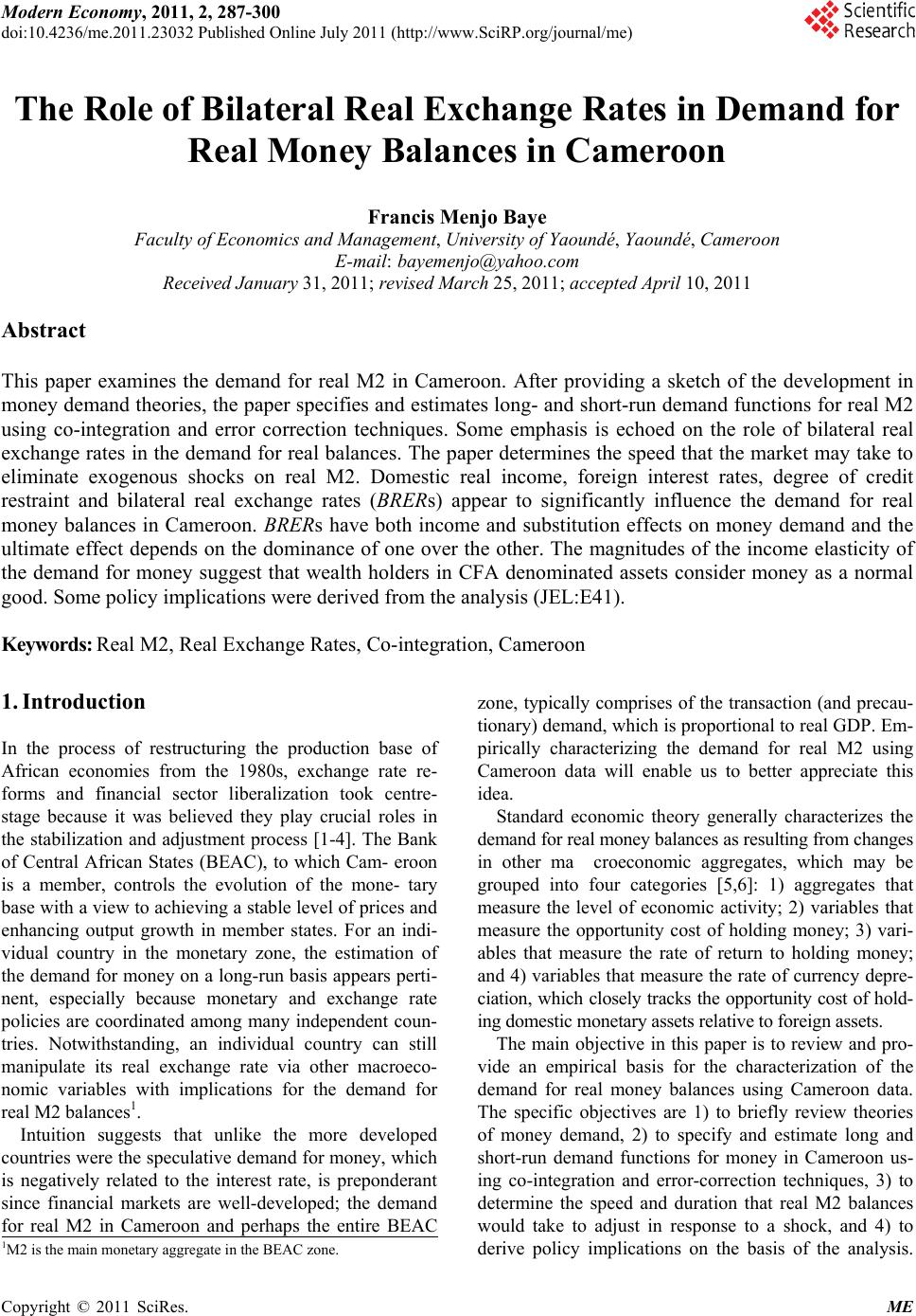
Modern Economy, 2011, 2, 287-300
doi:10.4236/me.2011.23032 Published Online July 2011 (http://www.SciRP.org/journal/me)
The Role of Bilateral Real Exchange Rates in Demand for
Real Money Balances in Cameroon
Francis Menjo Baye
Faculty of Economics and Management, University of Yaoundé, Yaoundé, Cameroon
Received January 31, 2011; revised March 25, 2011; accepted April 10, 2011
Abstract
This paper examines the demand for real M2 in Cameroon. After providing a sketch of the development in
money demand theories, the paper specifies and estimates long- and short-run demand functions for real M2
using co-integration and error correction techniques. Some emphasis is echoed on the role of bilateral real
exchange rates in the demand for real balances. The paper determines the speed that the market may take to
eliminate exogenous shocks on real M2. Domestic real income, foreign interest rates, degree of credit
restraint and bilateral real exchange rates (BRERs) appear to significantly influence the demand for real
money balances in Cameroon. BRERs have both income and substitution effects on money demand and the
ultimate effect depends on the dominance of one over the other. The magnitudes of the income elasticity of
the demand for money suggest that wealth holders in CFA denominated assets consider money as a normal
good. Some policy implications were derived from the analysis (JEL:E41).
Keywords: Real M2, Real Exchange Rates, Co-integration, Cameroon
1. Introduction
In the process of restructuring the production base of
African economies from the 1980s, exchange rate re-
forms and financial sector liberalization took centre-
stage because it was believed they play crucial roles in
the stabilization and adjustment process [1-4]. The Bank
of Central African States (BEAC), to which Cam- eroon
is a member, controls the evolution of the mone- tary
base with a view to achieving a stable level of prices and
enhancing output growth in member states. For an indi-
vidual country in the monetary zone, the estimation of
the demand for money on a long-run basis appears perti-
nent, especially because monetary and exchange rate
policies are coordinated among many independent coun-
tries. Notwithstanding, an individual country can still
manipulate its real exchange rate via other macroeco-
nomic variables with implications for the demand for
real M2 balances1.
Intuition suggests that unlike the more developed
countries were the speculative demand for money, which
is negatively related to the interest rate, is preponderant
since financial markets are well-developed; the demand
for real M2 in Cameroon and perhaps the entire BEAC
zone, typically comprises of the transaction (and precau-
tionary) demand, which is proportional to real GDP. Em-
pirically characterizing the demand for real M2 using
Cameroon data will enable us to better appreciate this
idea.
Standard economic theory generally characterizes the
demand for real money balances as resulting from changes
in other ma croeconomic aggregates, which may be
grouped into four categories [5,6]: 1) aggregates that
measure the level of economic activity; 2) variables that
measure the opportunity cost of holding money; 3) vari-
ables that measure the rate of return to holding money;
and 4) variables that measure the rate of currency depre-
ciation, which closely tracks the opportunity cost of hold-
ing domestic monetary assets relative to foreign assets.
The main objective in this paper is to review and pro-
vide an empirical basis for the characterization of the
demand for real money balances using Cameroon data.
The specific objectives are 1) to briefly review theories
of money demand, 2) to specify and estimate long and
short-run demand functions for money in Cameroon us-
ing co-integration and error-correction techniques, 3) to
determine the speed and duration that real M2 balances
would take to adjust in response to a shock, and 4) to
derive policy implications on the basis of the analysis.
1M2 is the main monetary aggregate in the BEAC zone.

F. M. BAYE 288
Section 2 of the paper charts out the monetary and ex-
change rate policy arrangements in the BEAC Zone. The
theoretical framework and literature review are presented
in Section 3. The methodology of the study is formulated
in Section 4. Section 5 presents the results, and a conclu-
sion is sketched in Section 6.
2. Monetary and Exchange Rate Policy
Arrangements in the Beac Zone
The BEAC Zone is a component of the wider Franc Zone
(FZ)2. It is governed by a number of principles: 1) use of
the same currency among members and hence, a com-
mon foreign exchange policy against the rest of the
world, 2) the reserves of the zone are pooled together,
and 3) there is full convertibility of the CFAF to the
EURO through the “Compte d’Operations” kept at the
French Treasury in which at least two-thirds of all for-
eign reserve earnings of member countries are held3.
These principles have far-reaching implications on the
economies of each of the member states. In the case of
Cameroon, monetary policy decisions are taken at the
level of BEAC and implemented by the national branch,
which is independent of the government4. This facilitates
the control of inflation in the region, though this might
be at the cost of output and employment objectives pur-
sued by the individual governments.
The fact that member countries are obliged to hold at
least two-thirds of their reserves in the “Compte
d’Operations” is quite constraining, yet a price to pay for
the full convertibility of the CFAF into the FF, and
through the FF to the EURO since January 2002. As a
group, the BEAC countries benefited from the discipline
imposed by the need to co-ordinate monetary policies
with member states. This, however, imposes constraints
on individual member countries. Some policies such as
monetary growth and nominal exchange rate changes
must be coordinated. This puts a greater burden on other
policy instruments for maintaining balance of payments
(BOP) equilibrium, particularly on fiscal and wage poli-
cies5. For an individual member to grapple well with
these policies, knowledge of the nature of the demand for
money could be helpful.
Real gross domestic product (GDP) growth in the FZ
was maintained at reasonable although not outstanding
rates compared to neighbouring non-CFA countries up to
1985 (for example, [8] and [9]). Growth collapsed in the
FZ from 1986, an outcome attributed to both the adverse
international environment and the accumulated effects of
poor domestic economic management. In addition to low
commodity prices, mounting debt, and economic mis-
management, the CFAF was severely over-valued
vis-à-vis other major currencies in the 1980s and the
early 1990s. The over-valuation eroded the profitability
and competitiveness of producing tradable goods, and
aggravated both financial and economic imbalances, as
well as long-standing structural problems [10]. The
chronic liquidity shortages in the African FZ among
other external factors led the two Central Banks on 2
August 1993 to suspend the repurchase of the CFAF
notes exported out of each of the sub-zones. This was
followed barely five months later by a 50% devaluation
of the CFA franc on January 12, 1994.
Cameroon, in particular, experienced an evolution
similar to that of other countries in the Zone. As showed
in Figure 1, it enjoyed a respectable annual growth rate
in real GDP of up to 12.5% in 1985. Growth collapsed
from 1986. Real output (measured by real GDP) in
Cameroon fell by 15.2% in 1987 and reached a depth of
18% in 1994, before climbing up to attain a positive 5.9%
annual growth rate in 1995 [11]. According to Figure 1,
growth in real M2 holdings and real GDP reached their
peak in 1985 before slowing down subsequently. Al-
though nominal M2 holdings grew 25-fold between 1968
and 1985, and 19-fold between 1968 and 1997, the aver-
age price level (as measured by the consumer price index)
0
100
200
300
400
500
70 75 80 85 90 95
Real M2
Real GDP
Bilateral RER with the US
Bilateral RER with Nigeria
Bilateral RER with France
Discount rate
2The African Franc Zone has three Central Banks: BEAC, (Banque des
Etats de l’Afrique Centrale) having as members, Cameroon, Chad,
Central African Republic, Congo, Equatorial Guinea and Gabon;
BCEAO (Banque Centrale des Etats de l’Afrique de l’Ouest), having as
members, Benin, Burkina Faso, Côte d’Ivoire, Mali, Niger, Senegal
and Togo; and the Central Bank of Comoros.
3See [7], for the situation of the entire Franc Zone.
4It could be recalled here that, the Board of Directors of BEAC is
composed of thirteen members―four representing Cameroon, three
France, two Gabon and one representing each of the other states.
5Critics of the African Franc Zone, observe that, the Franc Zone mone-
tary system lends itself to a spirit of laxity and contributes to the domi-
nation and exposure of the economies of member countries, and place
them at the mercy of any FF devaluation [7].
Figure 1. Evolution of real M2, real gdp, bilateral rers and
discount rate in cameroon (1968-1997). Source: Compiled
with data from the International Financial Statistics of the
IMF.

F. M. BAYE289
also grew over the entire period (not reported in Figure 1).
Once we divide nominal M2 by the price index to ob-
tain an index of real money holdings, Figure 1 shows
that real money balances grew only about 5-fold up to
1985 and 2-fold up to 1997 relative to 1968. Real GDP
rose 3.5-fold by 1985 and 2.4-fold by 1997 relative to its
level in 1968. Despite the observation that the opportu-
nity cost of holding money (surrogated by the discount
rate) doubled by 1985 relative to its value in 1968, the
growth in real M2 remained superior to that of real GDP
up to 1995. A priori, these observations appear to suggest
that in Cameroon, M2 holdings may tend to respond
more to GDP variations than to variations in the discount
rate. The construction of a real M2 schedule will enable
us to better understand this evolution. Bilateral real ex-
change rates with the United States appear to move with
real M2 and that with France tend to move in the oppo-
site direction, especially from 1980s. These tendencies
may become more apparent in the econometric analysis.
3. Conceptual Framework for Money
Demand and Literature Review
3.1. Conceptual Framework for Money Demand
In any economy, money plays at least four roles: 1) a
medium of exchange to facilitate the payment of income
and purchase of goods and services, 2) a unit of account -
measure by which all prices are established, 3) a store of
value - that alters the timing of spending decisions rela-
tive to earning income, and 4) a source of deferred pay-
ment. The two common measures of money as estab-
lished by monetary authorities in many developing coun-
tries are M1 and M2:
 M1 = Currency + Demand Deposits (checking ac-
counts or current accounts)
 M2 = M1 + Time Deposits (simple interest-bearing
savings accounts)
The first measure is known as the narrow definition of
money, which represents components that are readily
accepted as payments for goods and services or to satisfy
debts. The second measure is known as a broader defini-
tion, which includes savings accounts that can easily be
converted into currency or demand deposits. The mone-
tary authorities in the BEAC zone use M2 as the basic
monetary aggregate. We now turn to the classical money
demand theories.
3.1.1. The Classical Money Demand Theories
The classical economists insisted on Say’s law, which
states that “supply creates its own demand” and relegated
the role of money to the background. According to this
classical persuasion, money acts as a numéraire―a
commodity used in expressing prices and values, but
whose own value is unaffected by this role. In this regard,
money is “neutral” with no consequence for real eco-
nomic magnitudes and its role, as a store of value, is
perceived as limited under the classical assumption of
perfect information and negligible transaction costs [12].
Early theories of the demand for money can be traced
to the works of Mill, Walras, Jevons and Wicksell
[13-16]. The concept of demand for money took formal
shape through the quantity theory developed in the clas-
sical equilibrium framework by two different but equi-
valent expressions [17]. Irving Fisher of Yale University
provided the famous equation of exchange―MsVt = PtT
[18], where Ms represents quantity of money, Vt transac-
tions velocity of circulation, Pt prices and T the volume
of transactions―money is held simply to facilitate
transactions and has no intrinsic value per se.
An alternative theory―the so-called Cambridge ap-
proach or cash balance approach, is primarily associated
with the neo-classical economists such as Pigou and
Marshall [19,20] among others associated with the Cam-
bridge School. Their formulation is based on the simpli-
fying assumption that for an individual, the level of
wealth, the volume of transactions, and the level of in-
come-over short periods―would on the average move in
stable proportions to one another. They incorporated the
money market equilibrium conditions while invoking the
ceteris paribus clause to obtain the familiar quantity the-
ory formulation―MV = Py, which relates the quantity of
money to nominal income. In contrast with Fisher’s for-
mulation, V is now the “income velocity of circulation”
determined by technological and institutional factors and
is assumed to be stable. Given that the real income y is at
the full employment level and V being fixed, an increase
in the quantity of money results in a proportional in-
crease in P―that is, money is “neutral”―the familiar
quantity theory exposition.
The Cambridge formulation of the quantity theory
provides a more satisfactory description of monetary
equilibrium within the classical model [12]. It focuses on
the public’s demand for money, notably, the demand for
real money balances, as the important factor determining
the equilibrium price level that is consistent with a given
quantity of money. The emphasis the Cambridge formu-
lation places on the demand for money is remarkable
because it influences both the Keynesian and the Mone-
tarist theories.
3.1.2. Keynesian Theory
Keynes built upon the Cambridge approach to provide a
more rigorous analysis of money demand, focussing on
the motives for holding money [21,22]. Keynes postu-
lated three motives for holding money: transactions,

F. M. BAYE 290
precautionary and speculative purposes. He also formally
introduced the interest rate as another explanatory vari-
able influencing the demand for real cash balances.
In particular, 1) individuals will demand money to fi-
nance their daily purchases of goods and services, which
depends on the level of income; 2) individuals will de-
mand money as a contingency against unforeseen expen-
ditures, which also depends on the level of income; and 3)
individuals will hold money as a store of wealth, the
speculative motive6, which depends on the rate of inter-
est. The speculative or asset motive for holding money
arises because people dislike risk. Economic agents may
be prepared to sacrifice a high average rate of return to
obtain a portfolio with a low but more predictable rate of
return. Hence, individuals choose their portfolios to bal-
ance more certain but lower returns with higher but risk-
ier ones [24].
Since people hold money now in order to spend it later,
there is an obvious cost associated with holding money.
The opportunity cost of holding money is the interest
given up by holding money rather than financial assets7.
The transaction motive for holding money reflects the
fact that payments and receipts are not perfectly syn-
chronized8. Since the demand for money is viewed as the
demand for real money balances, a given amount of real
money is required to undertake a given quantity of total
transactions. Thus, when the price level doubles, in the
absence of monetary illusion, we expect the demand for
nominal money balances to double, leaving the de- mand
for real money balances unaltered.
3.1.3. Post-Keynes Theories
Following Keynes, a number of models were developed
to provide alternative explanations to confirm the for-
mulation relating real money balances with real income
and interest rates. These models can be classified into
three separate frameworks, namely: transactions, asset
and consumer demand theories of money [12,17]
Under the transactions theory of money demand fra-
mework, the inventory-theoretic approach [25,26] and
the precautionary demand for money [27] models were
introduced. These models were derived from the me-
dium-of-exchange function of money. The asset func-
tion of money led to the asset or portfolio approach
where major emphasis is placed on risk and expected
returns on assets [28].
Alternatively, the consumer demand theory approach
[29,30] considers the demand for money as a direct ex-
tension of the traditional theory of demand for any dura-
ble good. According to the Modern Monetarists view[31],
which is essentially a mere sophisticated version of the
Classical Quantity Theory, the demand for money is
necessary only to finance transactions, and it is consid-
ered as being related to a few key variables in a stable
manner. They argue that the demand for money is no
longer a function of solely the interest rate and income,
but that the rate of return on a much wider spectrum of
physical and financial assets would influence individu-
als’ demand for money. Accordingly, individuals will act
in such a way as to ensure that the rate of return at the
margin is equal across the complete range of physical
and financial assets that they could purchase. In this re-
gard, money is seen as a substitute for all other assets
and the demand for it is therefore a function of the rate of
return on all these assets.
Despite the different angles of the approaches to
money demand, it has been observed that real income
and the rate of interest or return constitute the main in-
gredients in the analyses of both the neoclassical and
variants of the neo Keynesian schools of thought [32].
The resulting implication of all the models is that the
optimal stock of real money balances is positively related
to real income and inversely related to the nominal rate
of return or interest. Although the different theories con-
sider similar key variables to explain the demand for
money, what sets them apart is that they frequently differ
in the specific role assigned to each. Notwithstanding,
one consensus that emerges from the literature is that
most empirical works are motivated by a blend of theo-
ries [33].
3.1.4. Derivation of the Basic Theoretical Model
As intimated earlier, economic agents typically hold cash
balances to allow for making transactions. The volume of
these transactions tends to be proportional to the aggre-
gate level of income. One approach to derive the func-
tional form of money demand, as discussed above, is
based on inventory control theory common in many
models of management. In this approach, optimal cash
balances are based on minimizing the total cost of hold-
ing these cash balances. This total cost has as key com-
ponents the cost of making transactions into or out of
cash, and the increasing opportunity cost of holding lar-
ger balances. This cost relationship can be expressed as
follows:


min CbYM Mi

(1 )
6Some authors consider the speculative demand for money as the rea
l
K
eynisian invention [23].
7Financial assets may take the form of bills, bonds, equities, and foreign
currency.
8Hendry and Ericsson observe that the transaction-demand theory is
based on the need for money to even out the differences between in-
come and expenditure streams [24].
where b = the cost of making a single cash transaction
(i.e., withdrawals from a checking or savings account or
conversion into stocks and bonds), Y = Income, i = a
market-determined interest rate or yield, M = the size of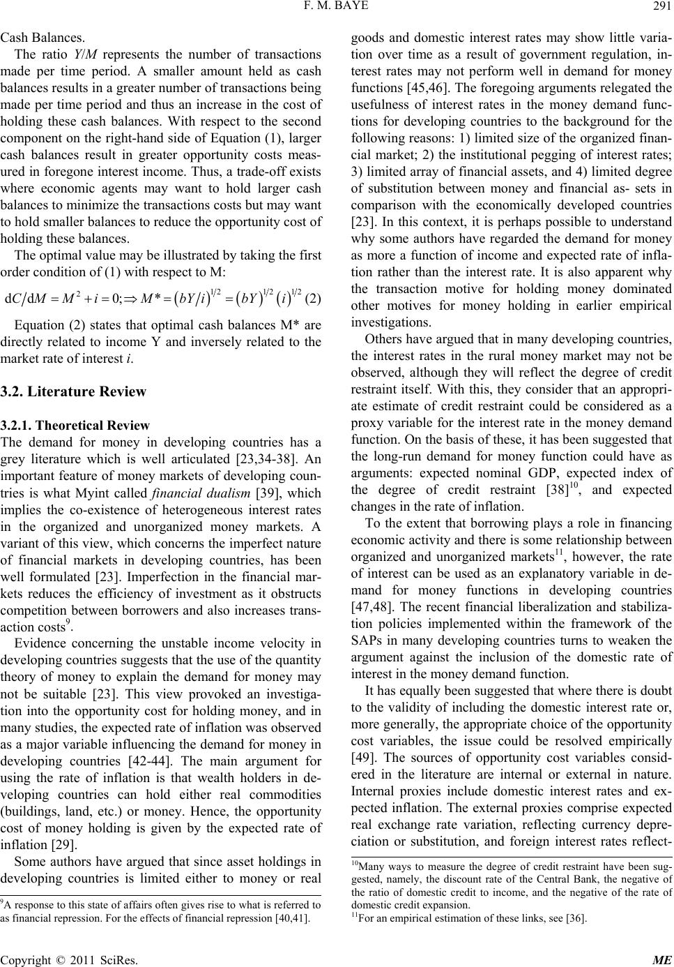

F. M. BAYE291
Cash Balances.
The ratio Y/M represents the number of transactions
made per time period. A smaller amount held as cash
balances results in a greater number of transactions being
made per time period and thus an increase in the cost of
holding these cash balances. With respect to the second
component on the right-hand side of Equation (1), larger
cash balances result in greater opportunity costs meas-
ured in foregone interest income. Thus, a trade-off exists
where economic agents may want to hold larger cash
balances to minimize the transactions costs but may want
to hold smaller balances to reduce the opportunity cost of
holding these balances.
The optimal value may be illustrated by taking the first
order condition of (1) with respect to M:

1212 12
2
dd0; *CM MiMbYibYi (2)
Equation (2) states that optimal cash balances M* are
directly related to income Y and inversely related to the
market rate of interest i.
3.2. Literature Review
3.2.1. Theoretical Review
The demand for money in developing countries has a
grey literature which is well articulated [23,34-38]. An
important feature of money markets of developing coun-
tries is what Myint called financial dualism [39], which
implies the co-existence of heterogeneous interest rates
in the organized and unorganized money markets. A
variant of this view, which concerns the imperfect nature
of financial markets in developing countries, has been
well formulated [23]. Imperfection in the financial mar-
kets reduces the efficiency of investment as it obstructs
competition between borrowers and also increases trans-
action costs9.
Evidence concerning the unstable income velocity in
developing countries suggests that the use of the quantity
theory of money to explain the demand for money may
not be suitable [23]. This view provoked an investiga-
tion into the opportunity cost for holding money, and in
many studies, the expected rate of inflation was observed
as a major variable influencing the demand for money in
developing countries [42-44]. The main argument for
using the rate of inflation is that wealth holders in de-
veloping countries can hold either real commodities
(buildings, land, etc.) or money. Hence, the opportunity
cost of money holding is given by the expected rate of
inflation [29].
Some authors have argued that since asset holdings in
developing countries is limited either to money or real
goods and domestic interest rates may show little varia-
tion over time as a result of government regulation, in-
terest rates may not perform well in demand for money
functions [45,46]. The foregoing arguments relegated the
usefulness of interest rates in the money demand func-
tions for developing countries to the background for the
following reasons: 1) limited size of the organized finan-
cial market; 2) the institutional pegging of interest rates;
3) limited array of financial assets, and 4) limited degree
of substitution between money and financial as- sets in
comparison with the economically developed countries
[23]. In this context, it is perhaps possible to understand
why some authors have regarded the demand for money
as more a function of income and expected rate of infla-
tion rather than the interest rate. It is also apparent why
the transaction motive for holding money dominated
other motives for money holding in earlier empirical
investigations.
Others have argued that in many developing countries,
the interest rates in the rural money market may not be
observed, although they will reflect the degree of credit
restraint itself. With this, they consider that an appropri-
ate estimate of credit restraint could be considered as a
proxy variable for the interest rate in the money demand
function. On the basis of these, it has been suggested that
the long-run demand for money function could have as
arguments: expected nominal GDP, expected index of
the degree of credit restraint [38]10, and expected
changes in the rate of inflation.
To the extent that borrowing plays a role in financing
economic activity and there is some relationship between
organized and unorganized markets11, however, the rate
of interest can be used as an explanatory variable in de-
mand for money functions in developing countries
[47,48]. The recent financial liberalization and stabiliza-
tion policies implemented within the framework of the
SAPs in many developing countries turns to weaken the
argument against the inclusion of the domestic rate of
interest in the money demand function.
It has equally been suggested that where there is doubt
to the validity of including the domestic interest rate or,
more generally, the appropriate choice of the opportunity
cost variables, the issue could be resolved empirically
[49]. The sources of opportunity cost variables consid-
ered in the literature are internal or external in nature.
Internal proxies include domestic interest rates and ex-
pected inflation. The external proxies comprise expected
real exchange rate variation, reflecting currency depre-
ciation or substitution, and foreign interest rates reflect-
10Many ways to measure the degree of credit restraint have been sug-
gested, namely, the discount rate of the Central Bank, the negative o
f
the ratio of domestic credit to income, and the negative of the rate o
f
domestic credit expansion.
11For an empirical estimation of these links, see [36].
9A response to this state of affairs often gives rise to what is referred to
as financial repression. For the effects of financial repression [40,41].

F. M. BAYE 292
ing substitution between domestic and foreign financial
assets. An increase in short-term foreign interest rates will,
ceteris paribus, induce domestic residents to substitute
foreign securities for domestic securities in their portfo-
lios, reducing their money holdings in the process [50].
3.2.2. Developments in Approaches to Money
Demand Estimation
The specification of money demand has spanned partial
adjustment modeling, buffer stock modeling and now
variants of co-integration and error correction modeling.
Partial adjustment models (PAMs) in a log-log functional
form was first applied to the demand for money by [51]
and later popularized by [52]. The PAM introduced two
concepts: 1) distinction between desired and actual
money holdings, and 2) the schemes by which the actual
money holdings adjust to the desired levels. This model
fared well in 1960s and early 1970s, but failed in captur-
ing the instability observed in the demand for money
from 1973 data. As such, PAMs were shown to suffer
from both specification problems and highly restrictive
dynamics [33]. To address these short-comings, two so-
lutions were proposed – modifying the theoretical under-
pinnings and improving the dynamic structure. The PAM
lost favor to buffer stock models (BSMs) in terms of the
modification of the theoretical bases [53], and to error
correction models (ECMs) in terms of improvements in
the dynamic structure. It has, however, been shown that
PAMs and BSMs are special cases of ECMs [54,55].
Proponents of the BSMs attributed the failings of the
PAMs to their inability to explicitly capture the short-run
impact of monetary shocks. Despite the appeal of BSMs
in explicitly modeling money shocks and using more
complex lag structures, they were equally accused of
suffering from empirical shortcomings [56]. As criticism
grew, the BSMs lost their appeal in favor of ECMs. In
the context of ECMs, 1) the data characteristics are
thoroughly examined before selecting the appropriate
estimation techniques, 2) lag structures are selected based
on data-generating processes of the economic variables
and not on a priori based on economic theory or some
naïve expectations, and 3) economic theory is allowed to
specify the long-run equilibrium while the short-run dy-
namics are defined from the data.
Two widely used error correction techniques have
been suggested [57-59]. The later approach provides an
opportunity to evaluate the presence of multiple co-inte-
grating vectors. The two variants of this approach―the
vector error correction models (VECM) and structural
time series models (STSM) are capable of jointly esti-
mating the long- and short-run components of the de-
mand for money [5]. In most cases, these modeling ap-
proaches become parameter intensive in estimating the
short-run autoregressive components, and most often
than not, there is little guidance from economic theory on
the appropriate lag structure to be selected. In this paper,
we use the Engle and Granger two-stage method because
it is simple to implement and all our variables are I (1).
Moreover, the original Engle-Granger framework is a
special case of multiple co-integrating vectors [57].
3.2.3. Empirical Review
Using annual data from 1948/49-1964/65 and in the case
of India, income proved to be the most significant deter-
minant of the demand for real cash balances, the interest
rate being statistically insignificant [35]. It was con-
cluded that the Indian money market was then compara-
tively underdeveloped. This outcome supported the con-
tention that the interest elasticity of the demand for
money function would be more significant in countries
with well developed money markets [34].
Simmons provides estimates of the demand for money
functions drawing on the “general-to-specific” approach
to modeling dynamic time series [49]. This approach is
associated with David Hendry and his followers [24,
60-62]. A lot of effort in the context of developed coun-
tries has recently been devoted to testing the stability of
the demand for money functions [63,64].
Following the lead of Adams [65], Atta and Anyangah
[66] present a more compre- hensive dynamic specifica-
tion of the general-to-specific approach, and observe that
1) domestic interest rates serve principally as a measure
of own rate of return on money, and 2) there is a margin
of substitution between money and securities denomi-
nated in foreign currencies in Botswana. Co-integration
and error correction mecha- nisms have also been used to
characterize the demand for money in a number of Afri-
can countries [67]. Cameroon is one of the four countries
included in the paper [67]. In the case of Cameroon, [67]
finds three co-integrating relationships among real broad
money, real GDP, infla- tion, interest rate and a measure
of price variability. His error-correction mechanism
passes the diagnostic tests and the error correction term
has a nearly unit coefficient. Recent endeavors at esti-
mating the demand for money functions are more meth-
odological than theory or policy- oriented. Empirical lit-
erature, which is policy oriented, on the demand for
money in Cameroon is scarce. It is one of our goals to
further reduce the extent of this scarcity.
4. Methodology of the Study
4.1. Econometric Model
A more general version of modeling the demand for real
money includes both real income, and the rate of interest

F. M. BAYE 293
[RERU, RERF, RERN] and all the variables are defined
in Table 1.
or the opportunity cost of money holdings as candidates
on the right-hand side as in Equation (3) (also see Equa-
tion 2). Following [50,68,69], we use the real exchange rate as
a proxy for expected currency depreciation. Changes in
the real exchange rate have two effects on the demand
for domestic currency―an income effect and a substitu-
tion effect. Assume that wealth holders evaluate their
portfolio in terms of domestic currency. Exchange rate
depreciation would increase the value of their foreign
asset holdings expressed in terms of domestic currency
and hence, be wealth enhancing. To maintain a fixed
share of their wealth invested in domestic assets, they
will repatriate part of their foreign assets to domestic
assets, including domestic currency. Hence, exchange
rate depreciation would increase the demand for domes-
tic currency.
,
d
MY
f
R
PP





(3)
where Md is desired money holding in nominal terms, P
the general price level, Y the GDP or national income in
nominal terms, and R a vector reflecting the opportunity
cost of money holdings. In the present endeavours, we
elect to specify a long-run money demand function and
then its short-run counterpart.
4.1.1. Long-Run Demand for Money
Drawing on the literature, we start by postulating a
long-run desired demand for real money balances as a
function of real income, a vector of opportunity costs for
money holdings, and a vector of bilateral real exchange
rates given by Equation (4).


 
01
,2 ,3
,,
log log
log log
d
t
t
ii
it it
MP YP
OPCOST RER

t



  
(4)
On the other hand, exchange rate movements may
generate a currency substitution effects in which invest-
tors’ expectation plays a crucial role. If wealth holders
develop an expectation that the exchange rate is likely to
deteriorate further following an initial depreciation, they
will respond by raising the share of their foreign assets in
their portfolios. In this context, currency depreciation
where (OPCOST)i  [DIR, CR, MMRG], (RER)i 
Table 1. Definition of variables.
Variable Definition
Md Desired stock of nominal cash balances (M2)
P General price level captured by the consumer price index (1990 = 100)
Y Nominal income represented by the GDP
(OPCOST)i A vector of the opportunity costs for money holdings.
DIR
Domestic interest rate represented by the discount rate of the Central Bank (BEAC)
The discount rate was used because of the absence of sufficient time series data on the lending and borrowing rates of
interest.
CR Degree of credit restraint captured by the ratio of GDP to domestic credit.
Wong (1977) suggested a similar measure for the degree of credit restraint.
MMRG
Money market rate of interest in Germany. It is believed that part of the currency flight or speculation from the CFA
countries was attributed to its full convertibility then, and the high interest rates in Germany before and after reunifica-
tion in 1990
(RER)i
A vector of bilateral real exchange rates. The bilateral real exchange rates were computed as: [nominal exchange rate
with country i]*[(consumer price index of country i)/ (consumer price index of Cameroon)]. An increase in the index
implies depreciation and a decrease an appreciation. The nominal exchange rate used is the period average, (line rf) in
the International Financial Statistics12.
RERU Bilateral real exchange rate with the Unites States.
RERF Bilateral real exchange rate with France.
RERN Bilateral real exchange rate with Nigeria.
 A stochastic disturbance term
S
ources: All data for this study were collected from several issues of the International Financial Statistics of the International Monetary Fund.
12Most of Cameroon’s exports are quoted in $US, and France and Nigeria are Cameroon’s major suppliers―France, by virtue of its economic and
p
olitical affiliations and Nigeria by virtue of its neighborliness.

F. M. BAYE 294
means higher opportunity cost of holding domestic
money, so currency substitution can be used to hedge
against such risk. In this logic, exchange rate deprecia-
tion would decrease the demand for domestic money.
The actual effect of exchange rate depreciation is there-
fore, an empirical issue because it depends on which of
the effects dominates.
An upward movement in foreign rates of interest en-
hances the attractiveness of foreign assets, and acts as
incentives to domestic residence to substitute foreign
assets for domestic ones in their portfolios. This will
reduce the demand for domestic money holdings.
Since Equation (4) is expressed in log-linear func-
tional form, the parameters

j (j = 1, 2, 3) are elasticities
of real cash balances with respect to the corresponding
variables. Economic theory suggests that 
1  0,

i,2  0,
and i,3 are to be determined empirically. The constant
term 
o captures the effects of changing transactions
costs and financial innovation over time.
4.1.2. Co-Integration and Error-Correction
Mechanism to the Short-Run Model
The general way of relating variables in the long-run
demand for money function to capture short-run adjust-
ments, in the context of time series data, is to specify a
flexible dynamic distributed lag model, which includes
an error-correction term from a co-integrating relation-
ship as in Equation (5)13.
 



1
0
2
,,
0
3
,,
0
4
1
1
log log
log
log
ˆ log
n
j
tt
j
n
ij itj
j
n
ij it j
j
n
j
j
tt
tj
j
MP kaYP
bOPCOST
cRER
dMP 












 



v
(5)
where ˆt

is the predicted residual term from a
co-integrating relationship estimated from the long-run
model (Equation (4)),
 is the coefficient of the er-
ror-correction term,  is the difference operator and vt is
the usual white nose. This procedure, due to [57], is valid
if, at least, a co-integrating relation exists among the
variables14. When this happens, the variables are said to
be co-integrated and error-correction terms exist to ac-
count for short-run deviations from the long-run equilib-
rium relationship implied by the co-integration.
Data used in this paper is defined in Table 1 and
sourced from several issues of the International Financial
Statistics of the IMF. Data were collected for the period
1968-2000. For the long-run models, reviews adjusted
the estimation sample to cover the period 1969-2000. For
the short-run model, due to the admission of lags of up to
order 4, the estimation sample was adjusted to 1974-
2000.
4.2. Estimation Procedures
4.2.1. Time Series Pre-Testing Procedure
All the variables in the model were tested for unit roots
by the Augmented Dickey-Fuller test to eliminate the
possibility of spurious regressions and to verify whether
they can be represented more appropriately as difference
or trend stationary processes. However, as argued in
[70,71], the mechanical transformation by differencing to
induce stationarity eliminates, in many cases, the long-
run information embodied in the original level form of
the variables. The error-correction model (ECM) de-
rived from the co-integrating equation by including the
lagged error-correction term reintroduces, in a statistic-
cally acceptable way, the long-run information lost
through differencing. The error-correction term stands
for the short-run adjustment to long-run equilibrium
trends15.
4.2.2. Model Estimation Procedures
We move from the estimation of a co-integrating
long-run estimate of Equation (4) (defined when (Md/P)t
= (M/P)t, because in the long-run variables are in their
steady-state) to the short-run error-correction model
(ECM) using the general-to-specific methodology16. We
follow the two-step procedure for estimating co-inte-
grated error-correction models as suggested by [57]. In
step one, the co-integrating regression is estimated by
ordinary least squares; and the residual series (if it turns
out to be I(0)) is lagged and included among the ex-
planatory variables in the second step to estimate the
error-correction mechanism in addition to the short- run
dynamic model. An important condition to ensure that
the OLS estimation of the co-integrating regression is
asymptotically optimal is that the errors should be
non-correlated [73,74].
13The single-equation error-correction model can be considered as a
generalization of the conventional stock adjustment model widely used
in the specification of the demand for money functions, and is consis-
tent with optimizing behavior of economic agents in a dynamic envi-
ronment as demonstrated by [55].
14[57] pointed out that, even though individual time series may be
non-stationary, linear combinations of them can be, because equilibriu
m
forces tend to keep such series together in the long-run.
15This term also opens up an additional channel of Granger causality so
far ignored by the standard causality tests [72], namely, the dynamic
causality in the Granger (temporal) sense. This issue is, however, not
explored in this paper.
16That is, Equation (5) as modified by the appropriate data generating
p
rocesses.

F. M. BAYE295
5. Results
5.1. Results of the Unit Root Test
All the variables in Table 2 present evidence of
non-stationarity at levels. Rejection of the unit root hy-
pothesis for the first difference of these variables sug-
gests that we are dealing with integrated processes of the
first order, that is, I(1) processes. Hence, the risk of using
the original Engle-Granger formulation is minimal.
5.2. Co-Integrated Long-Run Estimates
Table 3 presents the co-integrating long-run results that
emanate from the implementation of the Engle-Granger
first step OLS estimation. Two versions of Equation (2)
are estimated, Model 1―the unrestricted version and
Model 2―the restricted version. The unrestricted ver-
sion includes all the variables postulated in Equation (4)
and the restricted version excludes variables that behave
perversely and/or are non-significant. The discussion that
follows is centred on Model 2, which is preferred. The
discount rate and the bilateral real exchange rate with
Nigeria (RERN) do not qualify for inclusion in Model 2
as sanctioned by their signs and/or poor t-ratios.
The fit of the regression is good as given by 2 R =
97%, and the residuals show no sign of serial correlation
as indicated by the Breusch-Godfrey LM test statistic.
Residuals of the co-integrating regression are stationary
at their levels as shown by the ADF test statistic on the
residuals. Thus, indicating that at least one co-integrating
relation exists among the variables. All the explanatory
variables included in Model 2 are significant, at least, at
the 1 % level of committing a type I error.
The long-run real money demand elasticities with re-
Table 2. Unit root testing.
Variable ADF level ADF first
difference
Order of
integration
log(M/P)t –2.0995 –3.4515** I(1)
log(Y/P)t –2.4708 –3.2114** I(1)
log(DIR)t –1.6584 –5.6331*** I(1)
log(MMRG)t –2.4821 –4.8947*** I(1)
log(CR)t –1.5735 –5.1777*** I(1)
log(RERU)t –1.9602 –4.4999*** I(1)
Log(RERF)t –1.4463 –5.2254*** I(1)
Log(RERN)t –1.4387 –3.5694** I(1)
Note: the ADF critical values of –3.6852 and –2.9705 indicate significance
at the 1% (***), and 5% (**) levels, respectively. All the variables are as
defined previously and are expressed in natural logarithms.
spect to real income (Y/P), money market rate of interest
in Germany (MMRG), credit restraint (CR), bilateral real
exchange rate with the US (RERU), and bilateral real
exchange rate with France (RERF) are 87%, –10%,
–67%, 36%, and –51%, respectively, as reported in Ta-
ble 3. As Table 3 shows, the opportunity cost of real
money holdings as proxied by the degree of credit re-
straint (CR) and the money market rate of interest in
Germany have a negative and very highly significant
effect on real money holdings. Real income registers a
positive and very highly significant effect on real money
balances. The indication here is that growth in real in-
come would provoke an increase in the demand for real
cash balances, and economic agents consider real money
as a normal good.
Table 3. Co-integrated long-run estimates.The Dependent
Variable is real money balances (M/P)t.
Long-run
Variable
Model 1 Model 2
log(Y/P)t
0.9548***
(7.0038)
0.8688***
(12.7489)
log(DIR)t
0.0230
(0.1174) -
DUM*log(MMRG)t
–0.1379***
(–2.9390)
–0.0973***
(–5.1771)
log(CR)t
–0.6656***
(–5.9486)
–0.6712***
(–8.9019)
log(RERU)t
0.3788***
(2.7387)
0.3565***
(2.9918)
log(RERF)t
–0.3451
(–1.4989)
–0.5063***
(–3.3446)
log(RERN)t
–0.0679
(–0.9557) -
Constant –0.2345
(–0.2017)
0.5836
(0.9426)
R-squared 0.977 0.976
Adj. R-squared 0.969 0.971
SSR 0.1087 0.1135
F-statistic 127.67*** 187.40***
ADF ECT –4.8796*** –4.7311***
Breucsh-Godfrey
LM Test
3.6831
(P > 0.2259)
3.0516
(P > 0.2174)
RESET Test 1.1694
(P > 0.1585)
2.4180
(P > 0.1342)
ARCH Test 1.2685
(P > 0.2703)
0.1030
(P > 0.7508)
Sample (1968-2000) (1968-2000)
Adjusted Sample (1969-2000) (1969-2000)
Note: ***, ** and * indicate significance at the 1%, 5% and 10% levels, re-
spectively. DUM is a dichotomous dummy variable, taking the value 1 from
1986 to track down the period of economic crisis and massive capital flight
towards Germany, and 0 otherwise.

F. M. BAYE 296
The effects of the bilateral real exchange rate on real
M2 are mixed. While depreciation in Cameroon’s bilat-
eral real exchange rate with the United States (RERU)
would enhance the demand for real M2 balances, that
with France (RERF) would reduce the demand for real
money balances in the long-run. This is an indication that
as the degree of competitiveness in Cameroon enhances
vis-à-vis the United States, the tendency would be for
wealth holders who do business with the two countries to
substitute CFAF holdings for the dollar as exports are
encouraged. On the other hand, depreciation in Camer-
oon’s bilateral real exchange rate with France (RERF)
would encourage exports from Cameroon, which may
favor an expansion in holdings denominated in French
francs – thanks to the fixed convertibility between the
CFAF and the FF in the period under study. Indeed, the
CFAF and the FF (now EURO) can be considered inter-
changeable with CFAF-denominated assets. In other
words, the income effect of the BRER with the United
States dominates the substitution effect and the opposite
applies to BRER with France. The indication here is that
economic agents would prefer portfolios with assets de-
nominated in EURO if they expect a further devaluation
of the CFA franc.
5.3. Dynamic Adjustment and Error-Correction
Estimates
The results presented in Table 4 submit valuable dy-
namic elements to explain the short-run determinants of
real M2 balances in Cameroon, following the Engle-
Granger Error-Correction approach. Lags of up to order
4 of the first differences of the variables in Equation (5)
were tested, and the non-significant ones omitted. The fit
of the restricted Model is good (2
R=89 %). There is no
evidence on the presence of serial correlation as indi-
cated by the Breusch-Godfrey LM statistic and the per-
formance of all the other diagnostic statistics reported in
Table 4 responded favorably.
A crucial parameter in the estimation of ECM is that
associated with the error-correction term (ECT). As in-
timated earlier, it measures the degree of adjustment of
the actual real money balances with regard to its desired
long-run equilibrium level. The error-correction term of
–0.6982 is correctly signed17, and significant at the 1%
level. This is an indication that about 70% of shocks on
the demand for real M2 balances are corrected by the
“feed-back” effect annually (Table 4). The error-co-
rrection coefficient can be manipulated, in the context of
the error-correction specification, to derive the corre-
sponding adjustment speed in terms of the number
Table 4. Dynamic Error-Correction Estimates in the Engle-
Granger Sense. The Dependent Variable is the first differ-
ence of the log of real money balances (log(M/P)t)
Variable Short-run
Coefficients
ECTt-1
–0.6982***
(–4.2113)
log(Y/P)t
0.7853***
(6.8590)
DUM*log(MMRG)t-4 –0.0364*
(–1.7720)
log(CR)t
–0.5034***
(–7.8329)
log(RERU)t
0.2592***
(3.7426)
log(M/P)t-1
0.1703**
(2.1460)
R-squared 0.9129
Adj. R-squared 0.8888
SSR 0.0362
Breusch-Godfrey
LM Test
0.4515
(P > 0.6445)
RESET Test 0.0002
(P > 0.9893)
ARCH Test 1.0922
(P >0.3078)
Sample (1968-2000)
Adjusted Sample (1974-2000)
Note: ***, ** and * indicate significance at the 1%, 5% and 10% levels,
respecttively. ECT is the co-integrating error-correction term, and  is the
first difference operator.
of time periods required to eliminate a given exogenous
shock18. From our computations, in order to eliminate
95% of the effects of a shock on real M2 in Cameroon, it
would take about 2.5 years.
Our ECM suggests that the demand for real M2 in the
short-run is determined by the first differences of real
income; money market rate of interest in Germany, the
degree of credit restraint, bilateral real exchange rate
with the US, and the one-period-lagged dependent vari-
able. The bilateral real exchange rate with France has a
long-run effect on real M2 balances, but fails to exhibit
any short-run effect. The indication here is that in the
short-run the income effect may overshadow the substi-
tution effect of BRERs.
Short- and long-run elasticities of real money holdings
(M/P) with respect to real income (79%; 87%), market
rate of interest in Germany (–4%; –10%), degree of
18As explained by [102], adjustment periods can be computed as: (1 – a
= (1 –  )t, where t is the number of periods,  is the error-correction
coefficient and a = 0.95, if we want to estimate the approximate time
p
eriod needed to dissi
p
ate 95% of the effects of an exo
g
enous shock.
17The error-correction term has to remain negative for dynamic stability
[101].

F. M. BAYE297
credit restraint (–50%; –67%), RERU (26%; 36%), and
RERF (0%; –51%), respectively, are given in Tables 3
and 4. The most responsive of the determinants of the
demand for real M2 balances in the long-run appears to
be real income, followed by the degree of credit restraint
and Cameroon’s bilateral real exchange rate with the
United States.
6. Conclusions
An attempt has been made to provide an empirical basis
for the characterization of the nature of demand for
money in Cameroon. Specifically, the paper 1) undertook
a brief excursion in the development of money demand
theories, 2) specified and estimated demand functions for
money in Cameroon using co-integration and er-
ror-correction techniques, and 3) analyzed the speed that
may be taken by the local money market to absorb ex-
ogenous shocks on real M2 balances.
Domestic real income, foreign interest rates, degree of
credit restraint and bilateral real exchange rates were
found to significantly influence the demand for real
money balances in Cameroon during the period under
study. Bilateral real exchange rates have both income
and substitution effects on money demand and the ulti-
mate effect depends on the dominance of one over the
other. Domestic interest rates failed to manifest a sig-
nificant effect. The magnitudes of the short- and long-run
income elasticities of the demand for real M2 suggest
that wealth holders in CFA-denominated assets consider
money as a normal good.
The error-correction specification suggested an ad-
justment speed to long-run equilibrium of about 70 per
cent per annum, which indicates that about 95% of the
effects of any exogenous shock in real M2 balances in
Cameroon would take, on the average, about 2.5 years to
be eliminated.
The following policy implications emanated from our
results:
 by virtue of the rigidity of the nominal exchange rates
facing the CFA, implementing policies that will
dampen domestic prices, relative to those of trading
partners, could , at least in part, ameliorate the ability
of policy-makers to manipulate the demand for real
M2;
 if the objective is to sustainably enhance the demand
for real M2 balances, then narrowing the gap between
growth in GDP and that of domestic credit to the
economy, and vice versa, is worthwhile;
 there are benefits to be derived by monitoring money
market developments in main partner countries with a
view to supporting or countering potential tendencies
as regards currency substitution or speculation via
asset holdings, and
 policies geared towards influencing the demand-side
of the money market should be designed at least with
a medium term perspective.
7. References
[1] B. B. Aghevli and P. J. Montiel, “Exchange Rate Policies
in Developing Countries,” In: E.-M. Claassen, Ed., Ex-
change Rate Policies in Developing and Post-Socialist
Countries, International Center for Economic Growth,
San Francisco, 1990.
[2] S. Edwards, “Real Exchange Rate in Developing Coun-
tries: Concepts and Measurements,” In: T. J. Grennes, Ed.,
International Financial Markets and Agricultural Trade,
Westview Press, Boulder, 1990.
[3] I. A. Elbadawi, “Real Over-Valuation, Terms of Trade
Shock, and the Cost of Agriculture in Sub-saharan Af-
rica,” Policy Research Working Papers, WP 5831, The
World Bank, Washington, 1992.
[4] P. Arrau and J. de Gregorio, “Financial Innovation and
Money Demand: Application to Chile and Mexico,” Re-
view of Economics and Statistics, Vol. 75, No. 3, 1993,
pp. 524-530. doi:10.2307/2109469
[5] M. A. Cuevas, “Money Demand in Venezuela: Multiple
Cycle Extraction in a Co-Integration Framework,” Working
Paper, No. 2844, The World Bank, Washington, 2002.
[6] M. Bahmani-Oskooee and R. C. Wing Ng, “Long-Run
Demand for Money in Hong Kong: An Application of the
ARDL Model,” International Journal of Business and
Economics, Vol. 1, No. 2, 2002, pp. 147-155.
[7] A. M’Bet and A. M. Niamkey, “European Economic In-
tegration and the Franc Zone: The Future of the CFA
France after 1996,” Research Paper 19, AERC, Nairobi,
1993.
[8] World Bank “Adjustment in Africa: Reforms, Results and
the Road Ahead,” A World Bank Policy Research Report,
Washington, 1994.
[9] M. F. Baye, “The CFA Franc Devaluation: Rationale,
Consequences and Limitations for Cameroon,” University
of Yaoundé II, (Manuscript), 1995.
[10] S. Devarajan and L. E. Hinkle, “The CFA Franc Parity
Change: An Opportunity to Restore Growth and Reduce
Poverty,” The World Bank, Washington, 1994.
[11] The International Monetary Fund, “International Finan-
cial Statistics,” 1998.
[12] S. S. Sriram, “Theory of Demand for Money: A Survey
of Literature,” The Indian Economic Journal, Vol. 49, No.
1, 2001, pp. 103-115.
[13] J. S. Mill, “Principles of Political Economy,” John W.
Parker, London, 1848.
[14] L. Walras, “Elements d’Economie Politique Pure,” F.
Pichon, Paris, 1900.
[15] W. S. Jevons, “Money and the Mechanism of Exchange,”
D. Appleton, London, 1875.

F. M. BAYE 298
[16] K. Wicksell, “Lectures on Political Economy,” Transla-
tion by E. Classen, London, 1906.
[17] R. Katafono, “A Re-Examination of the Demand for
Money in Fiji,” Working Paper 2001/03, Reserve Bank
of Fiji, 2001.
[18] I. Fisher, “The Purchasing Power of Money,” Macmillan,
New York, 1911.
[19] A. C. Pigou, “The Value of Money,” The Quarterly Jour-
nal of Economics, Vol. 32, No. 1, 1917, pp. 38-65.
doi:10.2307/1885078
[20] A. Marshall, “Money, Credit and Commerce,” Macmillan,
London, 1923.
[21] J. M. Keynes, “A Treatise on Money,” Macmillan, Lon-
don, 1930.
[22] J. M. Keynes, “The General Theory of Employment, In-
terest, and Money,” Macmillan, London, 1936.
[23] S. Ghatak, “Monetary Economics in Developing Coun-
tries,” Macmillan, London, 1981.
[24] D. F. Hendry and N. R. Ericsson, “An Econometric
Analysis of UK Money Demand,” American Economic
Review, Vol. 81, No. 1, 1991, pp. 8-38.
[25] W. J. Baumol, “The Transactions Demand for Cash: An
Inventory Theoretic Approach,” The Quarterly Journal of
Economics, Vol. 66, No. 4, 1952, pp. 545-556.
doi:10.2307/1882104
[26] J. Tobin, “The Interest-Elasticity of Transactions Demand
for Cash,” The Review of Economics and Statistics, Vol.
38, No. 3, 1956, pp. 241-247. doi:10.2307/1925776
[27] K. Cuthbertson and D. Barlow, “Money Demand Analy-
sis: An Outline,” In: M. P. Taylor, Ed., Money and Fi-
nancial Markets, Basil Blackwell, Cambridge, 1991.
[28] J. Tobin, ‘Liquidity Preference as Behavior Towards
Risk,” The Review of Economic Studies, Vol. 25, No. 2,
1958, pp. 65-86. doi:10.2307/2296205
[29] M. Friedman, “The Quantity Theory of Money–A Re-
statement,” In: M. Friedman, Ed., Studies in the Quantity
Theory of Money, University of Chicago Press, Chicago,
1956.
[30] W. A. Barnett, “Economic Monetary Aggregates: An Ap-
plication of Index Number and Aggregation Theory,”
Journal of Econometrics, Vol. 14, No. 1, 1980, pp. 11-48.
doi:10.1016/0304-4076(80)90070-6
[31] M. Friedman, “Post-War Trends in monetary Theory and
Policy,” National Banking Review, Vol. 3, No. 1, 1964, pp.
1-9.
[32] D. E. W. Laidler, “The Demand for Money: Theories,
Evidence and Problems,” 4th Edition, Harper Collins
College Publishers, New York, 1993.
[33] S. S. Sriram, “A Survey of Recent Empirical Money De-
mand Studies,” IMF Staff Papers, Vol. 47, No. 3, 2001,
pp. 279-311.
[34] G. G. Kaufman and C. M. Latta, “The Demand for
Money; Preliminary Evidence from Industrial Countries,”
The Journal of Financial and Quantitative Analysis, Vol.
1, No. 3, 1966, pp. 75-89. doi:10.2307/233014
[35] D. Gujarati, “The Demand for Money in India,” Journal
of Development Studies, Vol. 5, No. 1, 1968, pp. 59-64
doi:10.1080/00220386808421282
[36] S. Ghatak, “Rural Money Markets in India,” Macmillan,
India, Delhi, 1976.
[37] S. Tomori, “The Demand for Money in the Nigerian
Economy,” Nigerian Journal of Economic and Social
Sciences, Vol. 14, No. 3, 1972, pp. 337-345.
[38] C. H. Wong, “Demand for Money in Developing Coun-
tries, Some Theoretical and Empirical Results,” Journal
of Monetary Economics, Vol. 3, No. 1, 1977, pp. 59-86.
doi:10.1016/0304-3932(77)90005-8
[39] H. Myint, “Economic Theory and the Underdeveloped
Country,” Oxford University Press, New York, 1971.
[40] R. I. McKinnon, “Money and Capital in Economic De-
velopment,” The Brookings Institute, Washington, 1973.
[41] E. S. Shaw, “Financial Deepening in Economic Devel-
opment,” Oxford University Press, New York, 1973.
[42] A. Hynes, “The Demand for Money and Monetary Ad-
justment in Chile,” Review of Economic Studies, Vol. 34
No. 3, 1967, pp. 285-293. doi:10.2307/2296676
[43] J. V. Deaver, “The Chilean Inflation and the Demand for
Money,” In: D. Meiselman, Ed., Variety of Monetary Ex-
perience, University of Chicago Press, Chicago, 1970, pp.
9-67.
[44] C. D. Campbell, “The Velocity of Money and the Rate of
Inflation; Recent Experiences in South Korea and Bra-
zil,” In: D. Meiselman, Ed., Variety of Monetary Experi-
ence, University of Chicago Press, Chicago, 1970, pp.
341-386.
[45] M. S. Khan, “Monetary Shocks and the Dynamics of
Inflation,” IMF Staff Papers, Vol. 27, No. 2, 1980, pp.
250-284. doi:10.2307/3866713
[46] M. J. Driscoll and A. K. Lahiri, “Income Velocity of
Money in Agricultural Developing Economies,” Review
of Economics and Statistics, Vol. 65, No. 3, 1983, pp.
393-401. doi:10.2307/1924184
[47] J. O. Adekunle, “The Demand for Money: Evidence from
Developed and Less Developed Economies,” IMF Staff
Papers, Vol. 15, 1968, pp. 220-266.
[48] Y. C. Parker, “The Variability of Velocity: An Interna-
tional Comparison,” IMF Staff Papers, Vol. 17, No. 30,
1970, pp. 620-637. doi:10.2307/3866361
[49] R. Simmons, “An Error-Correction Approach to Demand
for Money in Five African Developing Countries,” Jour-
nal of Economic Studies, Vol. 19, No. 1, 1992, pp. 29-47.
[50] S. Arango and M. I. Nadiri, “Demand for Money in Open
Economies,” Journal of Monetary Economics, Vol. 7, No.
1, 1981, pp. 69-83. doi:10.1016/0304-3932(81)90052-0
[51] G. C. Chow, “On the Long-Run and Short-Run Demand
for Money,” The Journal of Political Economy, Vol. 74,
No. 2, 1966, pp. 111-131 doi:10.1086/259130
[52] S. M. Goldfeld, “The Demand for Money Revisited,”
Brookings Papers on Economic Activity, Vol. 1973, No. 3,
1973, pp. 577-646. doi:10.2307/2534203
3

F. M. BAYE 299
[53] D. E. W. Laidler, “The ‘Buffer Stock’ Notion in Monetary
Economics,” The Economic Journal, Vol. 94, 1984, pp.
17-34. doi:10.2307/2232652
[54] D. F. Hendry, A. R. Pagan and J. D. Sargan, “Dynamic
Specification, Chapter 18,” In: Z. Griliches and D. Mi-
chael, Eds., Handbook of Econometrics, 2nd Edition, Vol.
1, Intriligator, New York, 1984, pp. 1023-1100.
[55] S. Nickell, “Error Correction, Partial Adjustment and all
that: An Expository Note,” Oxford Bulletin of Economics
and Statistics, Vol. 47, No. 2, 1985, pp. 119-130.
doi:10.1111/j.1468-0084.1985.mp47002002.x
[56] R. Milbourne, “Disequilibrium Buffer Stock Models: A
Survey,” Journal of Economic Surveys, Vol. 2, No. 3,
1988, pp. 187-208.
doi:10.1111/j.1467-6419.1988.tb00044.x
[57] R. Engle and C. W. J. Granger, “Co-integration and Er-
ror-Correction: Representation, Estimation, and Testing,”
Econometrica, Vol. 55, No. 2, 1987, pp. 251-276.
doi:10.2307/1913236
[58] S. Johansen, “Statistical Analysis of Cointegration Vec-
tors,” Journal of Economic Dynamics and Control, Vol.
12, No. 2-3, 1988, pp. 231-254.
[59] S. Johansen, K. Juselius, “Maximum Likelihood Estima-
tion and Inference on Cointegration―With Applications
to the Demand for Money,” Oxford Bulletin of Econom-
ics and Statistics, Vol. 52, No. 2, 1990, pp. 169-210.
[60] D. F. Hendry, “Econometrics–Alchemy or Science,” Eco-
nomica, Vol. 47, No. 188, 1980, pp. 387-406.
doi:10.2307/2553385
[61] C. L. Gilbert, “Professor Hendry’s Econometric Method-
ology,” Oxford Bulletin of Economics and Statistics, Vol.
48, No. 3, 1986, pp. 283-307.
doi:10.1111/j.1468-0084.1986.mp48003007.x
[62] A. Pagan, “Three Econometric Methodologies: A Critical
Appraisal,” Journal of Economic Surveys, Vol. 1 No. 1-2,
1987, pp. 3-24. doi:10.1111/j.1467-6419.1987.tb00022.x
[63] A. Beyer, “Modeling Money Demand in Germany,” Jour-
nal of Applied Econometrics, Vol. 13, No. 1, 1998, pp.
57-76.
doi:10.1002/(SICI)1099-1255(199801/02)13:1<57::AID-
JAE457>3.0.CO;2-Z
[64] E. Jondeau and N. Villermain-Lécolier, “La Stabilité de
la Fonction de Demande de Monnaie aux Etats-Unis,”
Revue Economique, No. 5, 1996, pp. 1121-1148.
[65] C. Adam, “Recent Developments in Econometric Methods:
An Application to the Demand for Money in Kenya,”
AERC Special Paper No. 15, 1992.
[66] J. K. Atta and J. Anyangah, “Dynamic Specification of
the Money Demand in Botswana,” African Journal of
Economic Policy, Vol. 4, No. 2, 1997, pp. 1-27.
[67] D. Fielding, “Money Demand in Four African Countries,”
Journal of Economic Studies, Vol. 21, No. 2, 1994, pp.
3-37. doi:10.1108/01443589410062968
[68] M. Bahmani-Oskooee and H. J. Rhee “Long-Run Elas-
ticities of the Demend for Money in Korea: Evidence
from Co-integration Analysis,” International Economic
Journal, Vol. 8, No. 2, 1994, pp 1-11.
[69] M. Bahmani-Oskooee and R. C. Wing Ng, “Long-run
Demand for Money in Hong Kong: An Application of the
ARDL Model,” International Journal of Business and
Economics, Vol. 1, No. 2, 2002, pp. 147-155.
[70] C. W. J. Granger, “Some Recent Developments in the
Concept of Causality,” Journal of Econometrics, Vol. 39,
No. 1-2, 1988, pp 199-211.
doi:10.1016/0304-4076(88)90045-0
[71] A. M. M. Masih and R. Masih, “Empirical Test to Dis-
cern the Dynamical Causality Chain in Macroeconomics
Activity: New Evidence from Thailand and Malaysia
Based on Multivariate Co-integrated VECM Approach,”
Journal of Policy Modeling, Vol. 18, No. 5, 1996, pp.
531-560. doi:10.1016/0161-8938(95)00133-6
[72] E. Kouassi, B. Decaluwe, C. M. Kapombe and D. Co-
lyer, “Temporal Causality and the Dynamic Interactions
betweeen Terms of trade and Current Account Deficits in
Co-integrated VAR Processes: Further Evidence from
Ivorian Time Series,” Applied Economics, Vol. 31, No. 1,
1999, pp. 89-96. doi:10.1080/000368499324589
[73] P. C. B. Phillips and M. Loretan, “Estimating Long-Run
Economic Equilibria,” Review of Economic Studies, Vol.
55, 1991, pp. 407-436. doi:10.2307/1913236
[74] I. A. Elbadawi and R. Soto, “Real Exchange Rates and
Macroeconomic Adjustments in Sub-Saharan Africa and
Other Developing Countries,” Journal of Africa Econo-
mies, Vol. 6, No. 3S, 1997, pp. 74-120.

F. M. BAYE 300
Appendix: List of Acronyms
BEAC: Banque des Etats de l’Afrique Centrale
(Bank of Central African States)
BRER: Bilateral Real Exchange Rate
BSMs: Buffer Stock Models
CFA: Currency of the members of the Franc
Zone
CR: Degree of Credit Restraint
ECMs: Error Correction Models
EURO: Currency of the European Union
FF: French Franc
FZ: Franc Zone
GDP: Gross Domestic Product
IFS: International Financial Statistics
M1: Currency plus Demand Deposits
M2: M1 plus Time Deposits
MMRG: Money Market Rate of Interest in Germany
PAMs: Partial Adjustment Models
RER: Real Exchange Rate
RERF: Bilateral Real Exchange Rate with France
RERN: Bilateral Real Exchange Rate with Nigeria
RERU: Bilateral Real Exchange Rate with the
United States
SAPs: Structural Adjustment Programmes
STSMs: Structural Time Series Models
US$: United States dollars
VECMs: Vector Error Correction Models