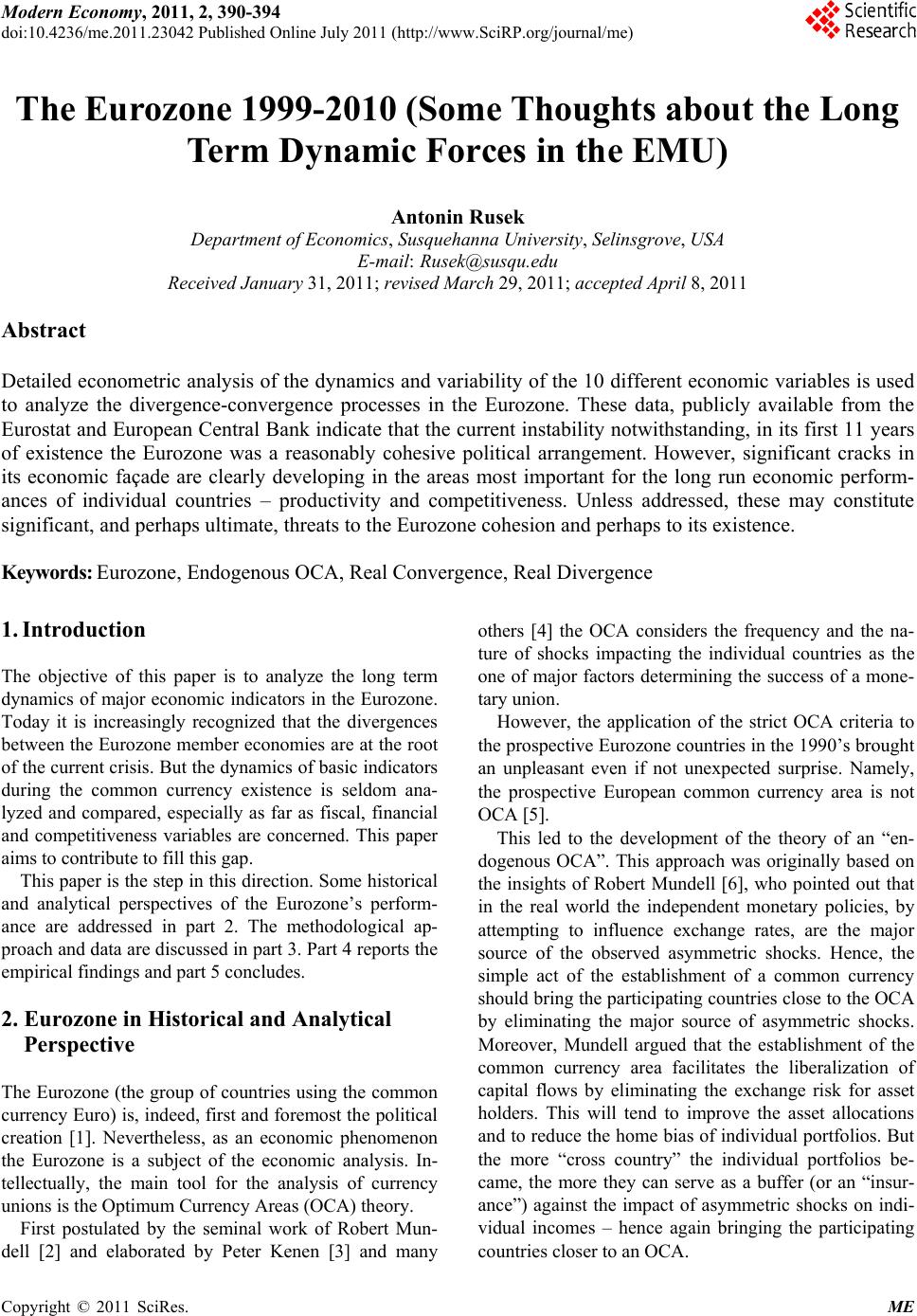Modern Economy, 2011, 2, 390-394
doi:10.4236/me.2011.23042 Published Online July 2011 (http://www.SciRP.org/journal/me)
The Eurozone 1999-2010 (Some Thoughts about the Long
Term Dynamic Forces in the EMU)
Antonin Rusek
Department of Economics, Susquehanna University, Selinsgrove, USA
Received January 31, 2011; revised March 29, 2011; accepted April 8, 2011
Abstract
Detailed econometric analysis of the dynamics and variability of the 10 different economic variables is used
to analyze the divergence-convergence processes in the Eurozone. These data, publicly available from the
Eurostat and European Central Bank indicate that the current instability notwithstanding, in its first 11 years
of existence the Eurozone was a reasonably cohesive political arrangement. However, significant cracks in
its economic façade are clearly developing in the areas most important for the long run economic perform-
ances of individual countries – productivity and competitiveness. Unless addressed, these may constitute
significant, and perhaps ultimate, threats to the Eurozone cohesion and perhaps to its existence.
Keywords: Eurozone, Endogenous OCA, Real Convergence, Real Divergence
1. Introduction
The objective of this paper is to analyze the long term
dynamics of major economic indicators in the Eurozone.
Today it is increasingly recognized that the divergences
between the Eurozone member economies are at the root
of the current crisis. But the dynamics of basic indicators
during the common currency existence is seldom ana-
lyzed and compared, especially as far as fiscal, financial
and competitiveness variables are concerned. This paper
aims to contribute to fill this gap.
This paper is the step in this direction. Some historical
and analytical perspectives of the Eurozone’s perform-
ance are addressed in part 2. The methodological ap-
proach and data are discussed in part 3. Part 4 reports the
empirical findings and part 5 concludes.
2. Eurozone in Historical and Analytical
Perspective
The Eurozone (the group of countries using the common
currency Euro) is, indeed, first and foremost the political
creation [1]. Nevertheless, as an economic phenomenon
the Eurozone is a subject of the economic analysis. In-
tellectually, the main tool for the analysis of currency
unions is the Optimum Currency Areas (OCA) theory.
First postulated by the seminal work of Robert Mun-
dell [2] and elaborated by Peter Kenen [3] and many
others [4] the OCA considers the frequency and the na-
ture of shocks impacting the individual countries as the
one of major factors determining the success of a mone-
tary union.
However, the application of the strict OCA criteria to
the prospective Eurozone countries in the 1990’s brought
an unpleasant even if not unexpected surprise. Namely,
the prospective European common currency area is not
OCA [5].
This led to the development of the theory of an “en-
dogenous OCA”. This approach was originally based on
the insights of Robert Mundell [6], who pointed out that
in the real world the independent monetary policies, by
attempting to influence exchange rates, are the major
source of the observed asymmetric shocks. Hence, the
simple act of the establishment of a common currency
should bring the participating countries close to the OCA
by eliminating the major source of asymmetric shocks.
Moreover, Mundell argued that the establishment of the
common currency area facilitates the liberalization of
capital flows by eliminating the exchange risk for asset
holders. This will tend to improve the asset allocations
and to reduce the home bias of individual portfolios. But
the more “cross country” the individual portfolios be-
came, the more they can serve as a buffer (or an “insur-
ance”) against the impact of asymmetric shocks on indi-
vidual incomes – hence again bringing the participating
countries closer to an OCA.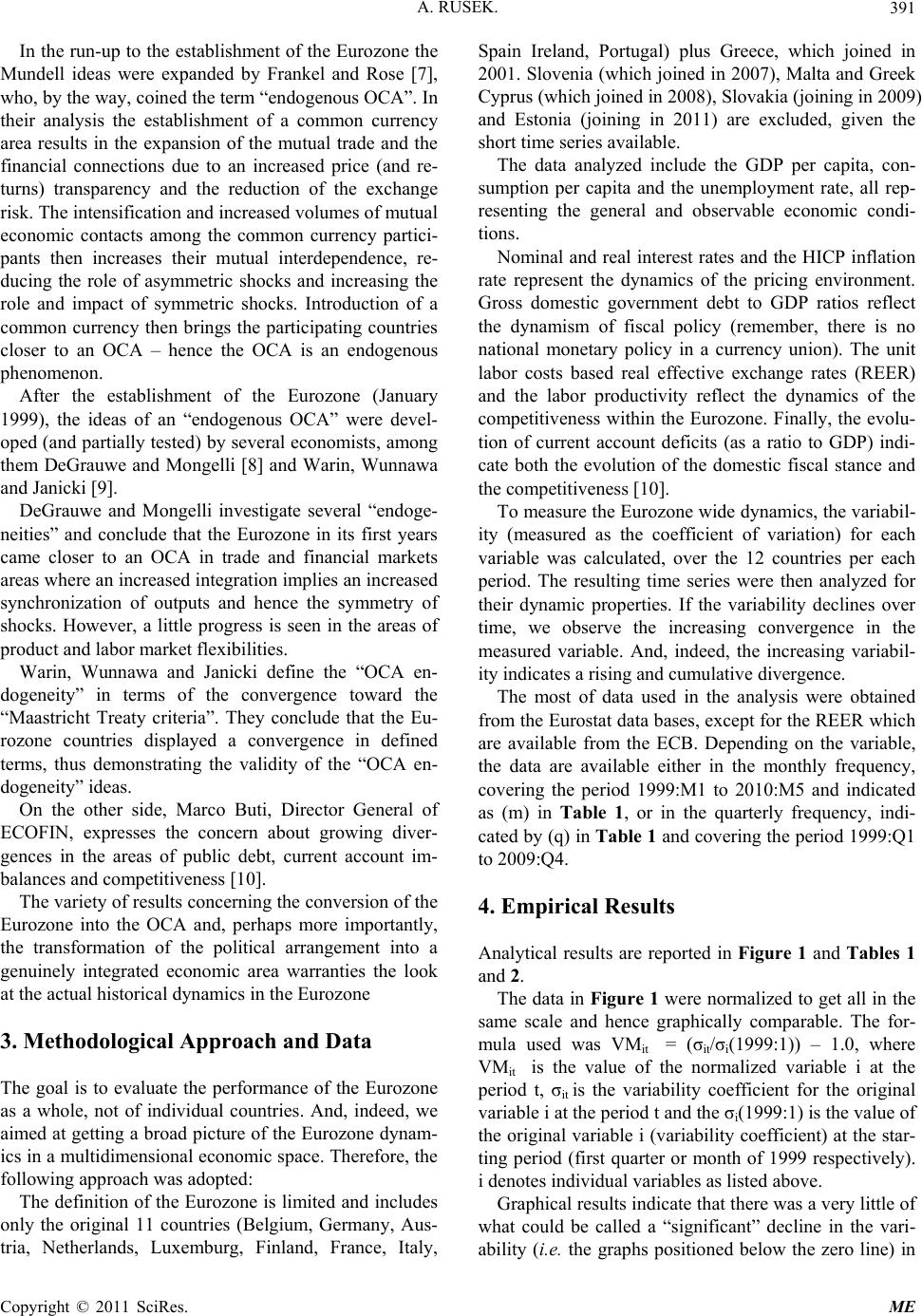

A. RUSEK.391
In the run-up to the establishment of the Eurozone the
Mundell ideas were expanded by Frankel and Rose [7],
who, by the way, coined the term “endogenous OCA”. In
their analysis the establishment of a common currency
area results in the expansion of the mutual trade and the
financial connections due to an increased price (and re-
turns) transparency and the reduction of the exchange
risk. The intensification and increased volumes of mutual
economic contacts among the common currency partici-
pants then increases their mutual interdependence, re-
ducing the role of asymmetric shocks and increasing the
role and impact of symmetric shocks. Introduction of a
common currency then brings the participating countries
closer to an OCA – hence the OCA is an endogenous
phenomenon.
After the establishment of the Eurozone (January
1999), the ideas of an “endogenous OCA” were devel-
oped (and partially tested) by several economists, among
them DeGrauwe and Mongelli [8] and Warin, Wunnawa
and Janicki [9].
DeGrauwe and Mongelli investigate several “endoge-
neities” and conclude that the Eurozone in its first years
came closer to an OCA in trade and financial markets
areas where an increased integration implies an increased
synchronization of outputs and hence the symmetry of
shocks. However, a little progress is seen in the areas of
product and labor market flexibilities.
Warin, Wunnawa and Janicki define the “OCA en-
dogeneity” in terms of the convergence toward the
“Maastricht Treaty criteria”. They conclude that the Eu-
rozone countries displayed a convergence in defined
terms, thus demonstrating the validity of the “OCA en-
dogeneity” ideas.
On the other side, Marco Buti, Director General of
ECOFIN, expresses the concern about growing diver-
gences in the areas of public debt, current account im-
balances and competitiveness [10].
The variety of results concerning the conversion of the
Eurozone into the OCA and, perhaps more importantly,
the transformation of the political arrangement into a
genuinely integrated economic area warranties the look
at the actual historical dynamics in the Eurozone
3. Methodological Approach and Data
The goal is to evaluate the performance of the Eurozone
as a whole, not of individual countries. And, indeed, we
aimed at getting a broad picture of the Eurozone dynam-
ics in a multidimensional economic space. Therefore, the
following approach was adopted:
The definition of the Eurozone is limited and includes
only the original 11 countries (Belgium, Germany, Aus-
tria, Netherlands, Luxemburg, Finland, France, Italy,
Spain Ireland, Portugal) plus Greece, which joined in
2001. Slovenia (which joined in 2007), Malta and Greek
Cyprus (which joined in 2008), Slovakia (joining in 2009)
and Estonia (joining in 2011) are excluded, given the
short time series available.
The data analyzed include the GDP per capita, con-
sumption per capita and the unemployment rate, all rep-
resenting the general and observable economic condi-
tions.
Nominal and real interest rates and the HICP inflation
rate represent the dynamics of the pricing environment.
Gross domestic government debt to GDP ratios reflect
the dynamism of fiscal policy (remember, there is no
national monetary policy in a currency union). The unit
labor costs based real effective exchange rates (REER)
and the labor productivity reflect the dynamics of the
competitiveness within the Eurozone. Finally, the evolu-
tion of current account deficits (as a ratio to GDP) indi-
cate both the evolution of the domestic fiscal stance and
the competitiveness [10].
To measure the Eurozone wide dynamics, the variabil-
ity (measured as the coefficient of variation) for each
variable was calculated, over the 12 countries per each
period. The resulting time series were then analyzed for
their dynamic properties. If the variability declines over
time, we observe the increasing convergence in the
measured variable. And, indeed, the increasing variabil-
ity indicates a rising and cumulative divergence.
The most of data used in the analysis were obtained
from the Eurostat data bases, except for the REER which
are available from the ECB. Depending on the variable,
the data are available either in the monthly frequency,
covering the period 1999:M1 to 2010:M5 and indicated
as (m) in Table 1, or in the quarterly frequency, indi-
cated by (q) in Table 1 and covering the period 1999:Q1
to 2009:Q4.
4. Empirical Results
Analytical results are reported in Figure 1 and Tables 1
and 2.
The data in Figure 1 were normalized to get all in the
same scale and hence graphically comparable. The for-
mula used was VMit = (σit/σi(1999:1)) – 1.0, where
VMit is the value of the normalized variable i at the
period t, σit is the variability coefficient for the original
variable i at the period t and the σi(1999:1) is the value of
the original variable i (variability coefficient) at the star-
ting period (first quarter or month of 1999 respectively).
i denotes individual variables as listed above.
Graphical results indicate that there was a very little of
what could be called a “significant” decline in the vari-
ability (i.e. the graphs positioed below the zero line) in n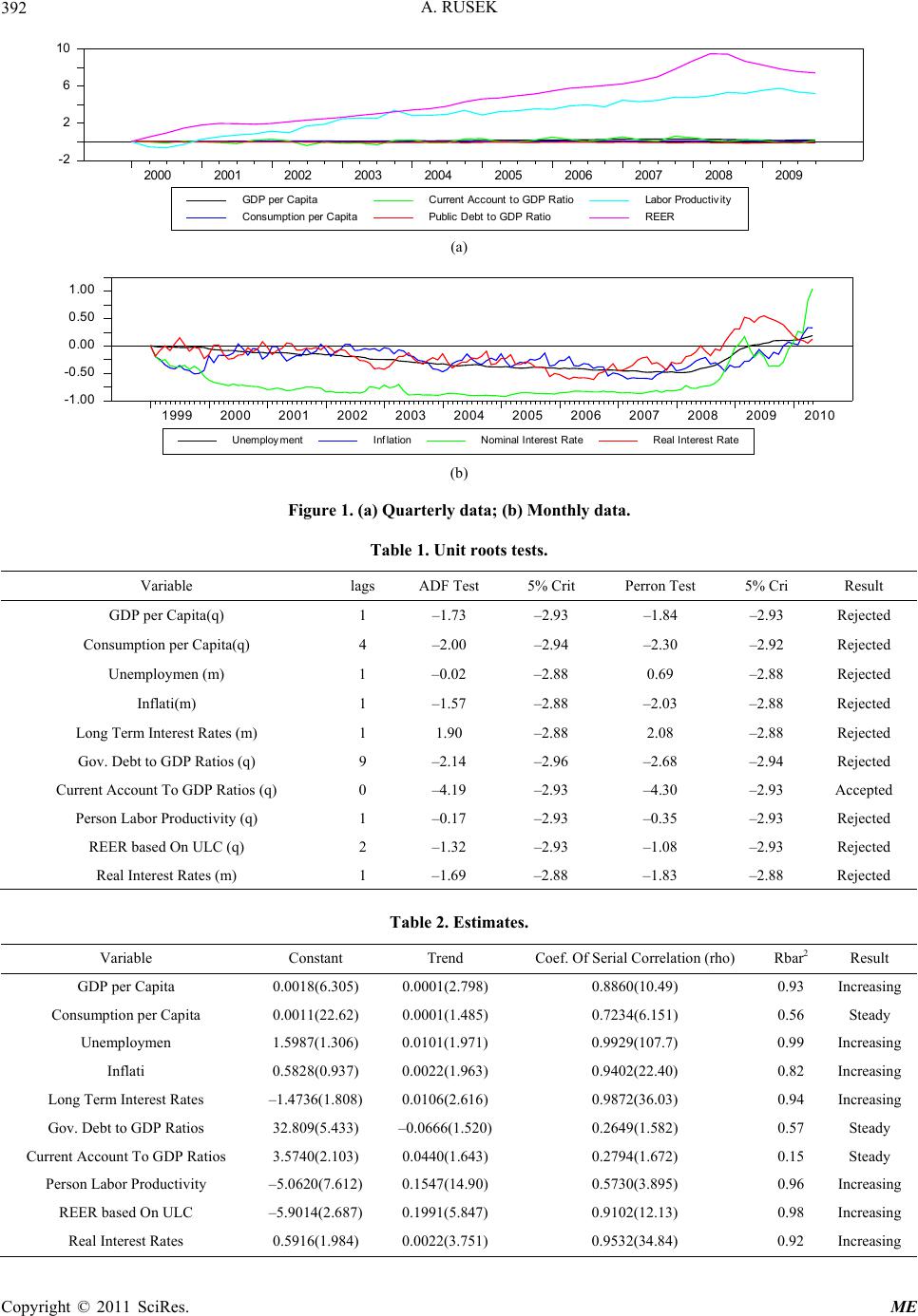

A. RUSEK 392
)Q y
GDP per Capi ta
C ons um pt i on per C apita
C urrent Ac c ount to GD P R at i o
Public Debt to GDP Ratio
Labor Produc t i vit y
REER
2000 2001 2002 2003 2004 2005 2006 2007 2008 2009
-2
2
6
10
(a)
Unemployment Inflation Nominal Interest RateReal Interest Rate
1999 2000 2001 2002 2003 2004 2005 2006 2007 2008 2009 2010
-1.00
-0.50
0.00
0.50
1.00
(b)
Figure 1. (a) Quarterly data; (b) Monthly data.
Table 1. Unit roots tests.
Variable lags ADF Test 5% Crit Perron Test 5% Cri Result
GDP per Capita(q) 1 –1.73 –2.93 –1.84 –2.93 Rejected
Consumption per Capita(q) 4 –2.00 –2.94 –2.30 –2.92 Rejected
Unemploymen (m) 1 –0.02 –2.88 0.69 –2.88 Rejected
Inflati(m) 1 –1.57 –2.88 –2.03 –2.88 Rejected
Long Term Interest Rates (m) 1 1.90 –2.88 2.08 –2.88 Rejected
Gov. Debt to GDP Ratios (q) 9 –2.14 –2.96 –2.68 –2.94 Rejected
Current Account To GDP Ratios (q) 0 –4.19 –2.93 –4.30 –2.93 Accepted
Person Labor Productivity (q) 1 –0.17 –2.93 –0.35 –2.93 Rejected
REER based On ULC (q) 2 –1.32 –2.93 –1.08 –2.93 Rejected
Real Interest Rates (m) 1 –1.69 –2.88 –1.83 –2.88 Rejected
Table 2. Estimates.
Variable Constant Trend Coef. Of Serial Correlation (rho) Rbar2 Result
GDP per Capita 0.0018(6.305) 0.0001(2.798) 0.8860(10.49) 0.93 Increasing
Consumption per Capita 0.0011(22.62) 0.0001(1.485) 0.7234(6.151) 0.56 Steady
Unemploymen 1.5987(1.306) 0.0101(1.971) 0.9929(107.7) 0.99 Increasing
Inflati 0.5828(0.937) 0.0022(1.963) 0.9402(22.40) 0.82 Increasing
Long Term Interest Rates –1.4736(1.808) 0.0106(2.616) 0.9872(36.03) 0.94 Increasing
Gov. Debt to GDP Ratios 32.809(5.433) –0.0666(1.520) 0.2649(1.582) 0.57 Steady
Current Account To GDP Ratios 3.5740(2.103) 0.0440(1.643) 0.2794(1.672) 0.15 Steady
Person Labor Productivity –5.0620(7.612) 0.1547(14.90) 0.5730(3.895) 0.96 Increasing
REER based On ULC –5.9014(2.687) 0.1991(5.847) 0.9102(12.13) 0.98 Increasing
Real Interest Rates 0.5916(1.984) 0.0022(3.751) 0.9532(34.84) 0.92 Increasing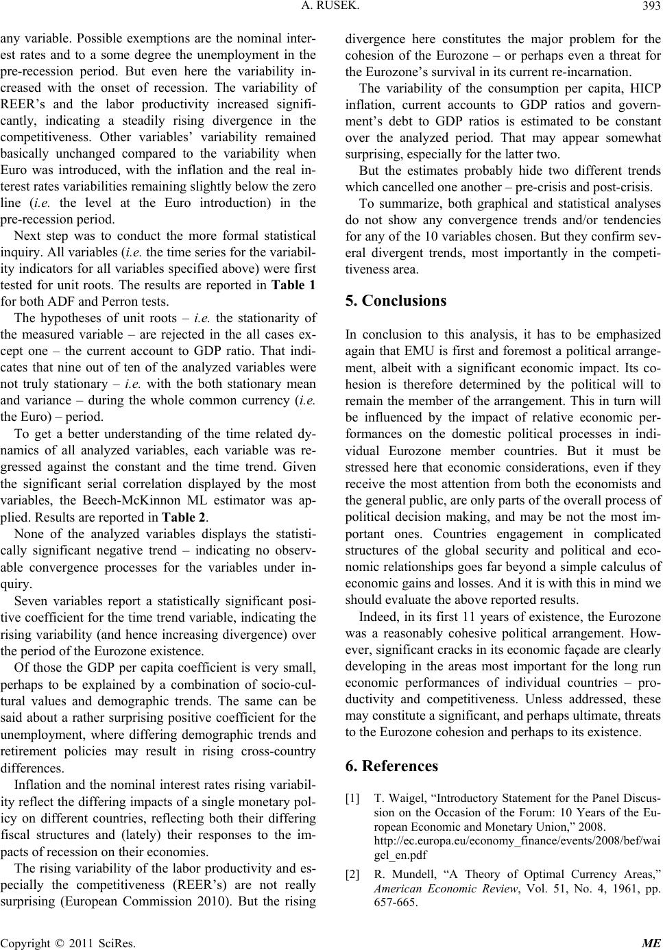

A. RUSEK. 393
any variable. Possible exemptions are the nominal inter-
est rates and to a some degree the unemployment in the
pre-recession period. But even here the variability in-
creased with the onset of recession. The variability of
REER’s and the labor productivity increased signifi-
cantly, indicating a steadily rising divergence in the
competitiveness. Other variables’ variability remained
basically unchanged compared to the variability when
Euro was introduced, with the inflation and the real in-
terest rates variabilities remaining slightly below the zero
line (i.e. the level at the Euro introduction) in the
pre-recession period.
Next step was to conduct the more formal statistical
inquiry. All variables (i.e. the time series for the variabil-
ity indicators for all variables specified above) were first
tested for unit roots. The results are reported in Table 1
for both ADF and Perron tests.
The hypotheses of unit roots – i.e. the stationarity of
the measured variable – are rejected in the all cases ex-
cept one – the current account to GDP ratio. That indi-
cates that nine out of ten of the analyzed variables were
not truly stationary – i.e. with the both stationary mean
and variance – during the whole common currency (i.e.
the Euro) – period.
To get a better understanding of the time related dy-
namics of all analyzed variables, each variable was re-
gressed against the constant and the time trend. Given
the significant serial correlation displayed by the most
variables, the Beech-McKinnon ML estimator was ap-
plied. Results are reported in Table 2.
None of the analyzed variables displays the statisti-
cally significant negative trend – indicating no observ-
able convergence processes for the variables under in-
quiry.
Seven variables report a statistically significant posi-
tive coefficient for the time trend variable, indicating the
rising variability (and hence increasing divergence) over
the period of the Eurozone existence.
Of those the GDP per capita coefficient is very small,
perhaps to be explained by a combination of socio-cul-
tural values and demographic trends. The same can be
said about a rather surprising positive coefficient for the
unemployment, where differing demographic trends and
retirement policies may result in rising cross-country
differences.
Inflation and the nominal interest rates rising variabil-
ity reflect the differing impacts of a single monetary pol-
icy on different countries, reflecting both their differing
fiscal structures and (lately) their responses to the im-
pacts of recession on their economies.
The rising variability of the labor productivity and es-
pecially the competitiveness (REER’s) are not really
surprising (European Commission 2010). But the rising
divergence here constitutes the major problem for the
cohesion of the Eurozone – or perhaps even a threat for
the Eurozone’s survival in its current re-incarnation.
The variability of the consumption per capita, HICP
inflation, current accounts to GDP ratios and govern-
ment’s debt to GDP ratios is estimated to be constant
over the analyzed period. That may appear somewhat
surprising, especially for the latter two.
But the estimates probably hide two different trends
which cancelled one another – pre-crisis and post-crisis.
To summarize, both graphical and statistical analyses
do not show any convergence trends and/or tendencies
for any of the 10 variables chosen. But they confirm sev-
eral divergent trends, most importantly in the competi-
tiveness area.
5. Conclusions
In conclusion to this analysis, it has to be emphasized
again that EMU is first and foremost a political arrange-
ment, albeit with a significant economic impact. Its co-
hesion is therefore determined by the political will to
remain the member of the arrangement. This in turn will
be influenced by the impact of relative economic per-
formances on the domestic political processes in indi-
vidual Eurozone member countries. But it must be
stressed here that economic considerations, even if they
receive the most attention from both the economists and
the general public, are only parts of the overall process of
political decision making, and may be not the most im-
portant ones. Countries engagement in complicated
structures of the global security and political and eco-
nomic relationships goes far beyond a simple calculus of
economic gains and losses. And it is with this in mind we
should evaluate the above reported results.
Indeed, in its first 11 years of existence, the Eurozone
was a reasonably cohesive political arrangement. How-
ever, significant cracks in its economic façade are clearly
developing in the areas most important for the long run
economic performances of individual countries – pro-
ductivity and competitiveness. Unless addressed, these
may constitute a significant, and perhaps ultimate, threats
to the Eurozone cohesion and perhaps to its existence.
6. References
[1] T. Waigel, “Introductory Statement for the Panel Discus-
sion on the Occasion of the Forum: 10 Years of the Eu-
ropean Economic and Monetary Union,” 2008.
http://ec.europa.eu/economy_finance/events/2008/bef/wai
gel_en.pdf
[2] R. Mundell, “A Theory of Optimal Currency Areas,”
American Economic Review, Vol. 51, No. 4, 1961, pp.
657-665.

A. RUSEK 394
[3] P. B Kenen, “The Theory of Optimum Currency Areas:
An Eclectic View,” In: R. Mundell and A. Swoboda, Eds.,
Monetary Problems of the International Economy, Chi-
cago University Press, Chicago, 1969, pp. 59-77.
[4] G. S. Tavlas, “The ‘New,’ Theory of Optimum Currency
Areas,” The World Economy, Vol. 16, No. 6, 1993, pp.
663-685.
[5] T. Bayoumi and B. Eichengreen, “Shocking Aspects of
European Monetary Unification,” In: F. Giavazzi and F.
Torres, Eds., Transition to Economic and Monetary Un-
ion in Europe, Cambridge University Press, New York,
1993, pp. 193-229.
[6] R Mundell, “Uncommon Arguments for Common Cur-
rencies,” In: H. Johnson and A. Swoboda, Eds., The
Economics of Common Currencies, Allen and Unwin,
London, 1973, pp. 114-132.
[7] J. A. Frankel and A. K. Rose, “The Endogeneity of the
Optimum Currency Area Criteria,” 1996.
http://www.nber.org/papers/w5700.pdf
[8] P. DeGrauwe and F. P. Mongelli, “Endogeneities of Op-
timum Currency Areas: What Brings Countries Sharing a
Single Currency Closer Together?” 2005.
http://www.ecb.europa.eu/pub/pdf/scpwps/ecbwp468.pdf
[9] T. Warin, P. V. Wunnava and H. P. Janicki, “Testing
Mundell’s Intuition of Endogenous OCA Theory,” Re-
vi ew of International Economics, Vol. 17, No. 1, 2009, pp.
74-86.
[10] European Commission, “Quarterly Report on the Euro
Area,” Economic and Financial Affairs, Vol. 1, No. 1,
March 2010, pp. 1-42.