Modern Economy, 2011, 2, 279-286
doi:10.4236/me.2011.23031 Published Online July 2011 (http://www.SciRP.org/journal/me)
Duration Dependence in Bull and Bear Stock Markets
Haigang Zhou, Steven E. Rigdon
1Department of Fin anc e, Clevela n d S t ate Universit y, Cleveland, USA
2Department of Mathem at i c s an d St at i st i cs , Southern Illinois University Edwardsville, Edwardsville, USA
Received January 20, 2011; revised March 15 , 20 1 1; accepted April 1, 2011
Abstract
Testing duration in stock markets concerns the ability to predict the turning points of bull and bear cycles.
The Weibull renewal process has been used in previous studies to analyze duration dependence in economic
and financial cycles. A goodness-of-fit test, however, shows that this model does not fit data from U.S. stock
market cycles. As a solution, this study fits the modulated power law process that relies on less restrictive
assumptions. Moreover, it measures both the long term properties of bull and bear markets, such as the ten-
dency of the cycles to become shorter (or longer), as well as the short term effects, such as duration depend-
ence. The results give evidence of negative duration dependence in all samples of bull markets and evidence
of positive duration dependence in complete, peacetime and post WWII samples of bear markets. There is no
evidence of any structural change in duration dependence after WWII in either bull or bear markets. The re-
sults show that bull and bear markets tend to get progressively shorter, but for bull markets this trend has
accelerated since WWII whereas for bear markets this trend has decelerated since WWII. Goodness-of-fit
tests suggest that the modulated power is a suitable model for U.S. stock market cycles.
Keywords: Modulated Power Law Process, Business Cycles, Financial Cycles, Power Law Process, Weibull
Distribution, Renew al Proc es s
1. Introduction
The duration dependence of stock market cycles can help
to pinpoint the peaks and troughs in these cycles. The
predictability o f turning po ints and the relevan ce of dura-
tion dependence analysis in financial markets has been
studied in [1] and [2]. Unstructured statistical models
have been used in modeling duration dependence in
business cycles [3], REOIT cycles [1], and stock market
cycles [2] and [4].
Previous studies have often used the Weibull renewal
process to study duration dependence in business and
financial cycles. For the Weibull renewal process, the
probability of an event in a small interval depends only
on the time since the previous event, and not on the pre-
vious pattern of failures or the times since the process
initially began. In particular, this model assumes that
after the occurrence of an event, the system is always in
exactly the same condition, precluding the possibility of
a long term change in the system. Through goodness-of-
fit tests, it was shown in [4] that U.S. business cycles do
not fit the simple Weibull renewal process model.
The nonhomogeneous Poisson process (NHPP) is ano-
ther model that has been used to odel the occurrence of
events in time. For an NHPP, the prob ability of an ev ent
in a small interval is some function of time since the ini-
tial startup of the system. An event and the subsequent
restarting of the system, therefore, has no effect on the
system performance. If the probab ility of an ev ent occur-
ring in a small interval is constant across time, then the
process is a homogeneous Poisson process where the
times between events are independent and identically
distributed exponential random variables. This special
case is also a renewal process.
Thus, for a renewal process, the system starts anew
each time there is an event, whereas for the NHPP, the
process picks up right where it left off. In the reliability
context, the renewal process is described as a good-as-
-new, or same-a s - new model, and the NHPP is described
as a bad-as-old or same-as-old model. Therefore, a
renewal process can model duration dependence but
not any long term effects, such as the tendency of in-
tervals to get longer or shorter. The NHPP, on the other
hand, can model long term effects, but not duration de-
pendence.
We propose using the modulated power law process

H. G. ZHOU ET AL. 280
(MPLP) to model duration dependence for U.S. stock
market cycles. This model, suggested by [5,6], and [7], is
a compromise between a renewal process and an NHPP.
With the MPLP, we are able to estimate long term effects,
such as events becoming progressively more (or less)
frequent, as well as short term effects, such as duration
dependence.
Our study is also related to the Frisch-Slutsky para-
digm of cycles. Frisch [8] and Slutsky [9] state that there
is no need to appeal to specific determinant causes of
cycles. Many of the advances in theories of cyclical vo-
latilities are in the field of business cycles and little
theoretical work has been devoted to financial cycles.
Although much of the following discussion on theories
of cycles are from business cycles, we believe that the
insight from the theories can also improve our under-
standing of financial cycles, even without identifying the
exact sources of shocks to the financial markets. Much
progress has been made in understanding business cycles
and even economists are not able to agree on the causes
of cyclical volatility. The exact cau ses of cyclical volatil-
ity are debated and identifying the sources of shocks to
the financial markets is beyond the scope of this study.
[10] provides a detailed review on the evolution of busi-
ness cycle theories. References [11] and [12] provide a
framework to identify shocks to the financial sectors.
Frisch [8] and Slutsky [9] argued that many phenomena
existed that could precipitate a real shock in the market’s
equilibrium path. A large negative shock, although rare,
would be sufficient to draw the average market activity
away from the equilibrium level for a sufficiently long
period of time to be considered a downswing. Slutsky
argued that “clusters” of small negative shocks can also
move the market away from its equilibrium. As we de-
scribe in Section 2.2, the MPLP involves one parameter
which can be thought of as the accumulated number of
shocks.
We fit the modulated power law process do data from
bull and bear markets. We consider separately peacetime
and war time data, as well as pre- and post-WWII data.
We find evidence of negative duration dependence in all
samples of bull markets and in pre-WWII bear markets,
and evidence of positive duration dependence in com-
plete, peacetime, and post-WWII samples of bear mar-
kets. In regards to the long term effect, evidence shows
that bull and bear markets tend to get progressively
shorter, but for bull markets, this trend has accelerated
since WWII, whereas for bear markets, this trend has
decelerated since WWII.
Section 2 describes the methodology used in the study
as well as the sampling data. Section 3 presents descrip-
tive statistics and empirical results, while Section 4 of-
fers concluding remarks.
2. Methodology and Data
In this study, both the Weibull renewal process and the
MPLP are used to examine the duration of bull and bear
markets. The Weibull renewal process and its variations
are widely used in the duration dependence literature.
The Weibull renewal process assumes a linear relation-
ship between the log of the intensity function (measured
from the last event and restart of the system) and that of
the durations. The MPLP is a generalization of both the
Weibull renewal process and the NHPP with a power law
intensity function. When we consider bull markets, we
ignore the intervening bear markets and treat the intere-
vent times as if they were back-to-back. Bear markets are
treated similarly.
2.1. Weibull Renewal Process
The Weibull renewal process assumes that the times be-
tween events are independent random variables, each
with the same Weibull distribution. The probability den-
sity function (PDF) and the hazard function for the Wei-
bull distribution are

1exp, 0,
tt
ft t


 

 



 

 

and




1
,0
1
ft t
ht t
Ft




 .




Here 0

 is a shape parameter and

is a scale
parameter. The hazard function is increasing when
1

, decreasing when 1


, and constant when 1


.
1
When


, Weibull distribution reduces to the
exponential distribution.
the
)
)
An increasing hazard function ( implies that
the conditional probability of a turning point in the mar-
ket cycle will thus increase as the duration of the cycle
increases; this indicates positive duration dependence.
On the other hand a decreasing hazard function
1  
(1


implies that the conditio nal probability of a turning point
will decrease as the duration of the cycle increases; this
indicates negative duration dependence.
We fit the Weibull renewal process to the bull and
bear markets from 1885 to 2000. Goodness-of-fit tests
reject the hypothesis of a Weibull renewal process for
both the bull markets and the bear markets. Further
details regarding the analysis of these data are found in
Section 3.2.
2.2. The Modulated Power Law Process
The MPLP was introduced by [5] and [6] as a compro-

H. G. ZHOU ET AL.281
mise between the Weibull renewal process and an NHPP
with intensity function

1,
t
t







 0,t
(1)
where time is measured from the initial startup of th e
system. The NHPP with this parametric form of the in-
tensity function is called the power law process in the
reliability literature. As we mentioned in Section 1, the
Weibull renewal process can be thought of as a same-
-as-new model, whereas the NHPP is a same-as-old
model because of the assumptions about what happens
after an event and restart of the system.
t
The MPLP is then derived as follows. Suppose that
shocks occur according to the power law process, the
NHPP with intensity function given in (1). Suppose fur-
ther that an event does not occur at every shock, but ra-
ther after every

shocks. For now we assume that

is a positive integer. After the

th shock, the shock
counter is reset to zero, but time t is not reset to zero.
This is what allows us to model the long term effects,
such as the tendency of times between events to increase.
For example, suppose that 2


and 5


t
; then we
would observe that shocks occur more and more fre-
quently as time advances, because the intensity function
for the shocks is proportional to , an increasing
function in . However, each time an event occurs, the
shock counter would be reset, so we would have positive
duration dependence. Thus, we would have positive du-
ration dependence while the long term tendency is to
have shorter durations. Larger values of
21
t

t

indicate
stronger positive duration dependence, whereas larger
values of indicate a long term tendency for shorter
and shorter intervals between events.

Since we consider the bull markets (and also the bear
markets) as if they were back-to-back, we let i denote
the time of the ith event, measured from the initial point
of data collection. We define 0. The interevent
times, 1iii
T
0T
X
TT

 , then represent the length of each
bull (or bear) market.
It can be shown (see, for example, [6,7]) that the ran-
dom variables
1,1,2,, ii
iTT ,
X
in



 
 
 
 
are independent and identically distributed random vari-
ables having a gamma distribution with PDF

 
1exp ,0.
x
fxx x





From this result, we can determine the likelihood
function for the i
X
’s, and then the likelihood function
for the observed ’s. Note that the ’s are the event
times measured from the initial startup of the system.
The log likelihood function is then
i
Ti T





12
1
1
1
,,,, ,lnln
ln1 ln
1ln
n
n
n
i
i
n
ii
i
t
tt tnn
nt
tt



 

 





 



 



(2).
The maximum likelihood estimates can then be ob-
tained by differentiating the log-likelihood function with
respect to each parameter, setting the results equal to
zero, and using a numerical method to approximate the
solution.
The description above relies on counting the number
of shocks to the system, requiring that

be a positive
integer. However, the likelihood in (2) is a valid likeli-
hood for all positive values of

, not just for positive
integers. The following example suggests how noninte-
ger values can be allowed for

. Suppose that local
events occur at the rate


t 
5
. Each time a local event
occurs, the probability that it is a shock to the system is
1/2. Suppose also, that


shocks will cause a sys-
tem event (end of bull/bear market). Since only about
half of the local events will cause a shock, there will be
on average


125 2.5 shocks that cause a failure.
The model just described is indistinguishable from a
MPLP with rate


t  and 2.5

. Other fractional
values can be similarly explained. In looking at another
way of explaining fractional values of

, [7] simulated
a number of processes for various values of

. They
found that with large values of

, the event times were
evenly spaced, possibly with a long term effect of inter-
event times getting shorter or longer. Thus for large

,
as the duration gets longer, we get closer to the next
point in the spacing, which means that the conditional
probability of a system event gets larger. For 1


, the
events are very much clustered, with a few very short
interevent times and a few very long interevent times.
These are much more clustered than would be expected
by a Poisson process. The existence of clustering sug-
gests negative duration dependence, since as the duration
increases, it becomes more likely that it is one of the
very long interevent times. For a third way of consider-
ing fractional valu es of

, we consider special cases of
the MPLP. When 1


, the MPLP with parameters

and

is a NHPP with intensity function


t 


1,t 
 
0t. When , then the MPLP with
parameters 1


and

is a Weibull renewal process.
Since noninteger values of

are allowed in the Wei-
bull distribution, it seems reasonable to allow noninteger
values in a generalization of the Weibull renewal process.

H. G. ZHOU ET AL. 282
time samples. The results indicate that war does not have
significant impact on the duration of stock markets. This
differs from the results reported in [4] that the average
length of the complete sample of expansions is lower
than that of peace time expansions. We also observe that
the average duration of bull markets is longer and the
average duration of bear markets is shorter in the
post-WWII subsample than in the pre-WWII subsample.
Finally, if , then the MPLP reduces to the ho-
mogeneous Poisson process with intensity function
1  

1t

 .
2.3. Data
Data from stock market cycles exist as far back as 1885.
These data, taken from [13], are reproduced in Table 1.
The bull and bear markets during wars are indicated in
bold face. Figure 1 shows plots of durations for bull and
bear markets both pre- and post-WWII. 3.2. Empirical Results from the Weibull Analysis
Table 3 shows the maximum likelihood estimates of the
parameters, along with confidence intervals. For bull
markets, the MLE for

is for the complete
sample. Because the 95% confidence interval excludes 1,
we conclude that there is evidence that the true value of
ˆ1.836
 

exceeds 1. This indicates that positive duration de-
pendence exists in cycles of bull markets. Similar results
are obtained for the peace time, and pre- and post-WWII
data (both bull and bear markets), supporting the exis-
tence of positive duration dependence. This implies that
the probability of a bull/bear market ending increases as
the duration increases. These results differ from those
3. Empirical Findings
3.1. Descriptive Statistics
Descriptive statistics of bull and bear markets, broken
down into peacetime, pre-WWII, and post-WWII are
reported in Table 2. The complete sample includes all
observations, while the peacetime sample excludes
war-time cycles. The average duration of bull markets is
28 months for the complete sample, and it is 27 months
for the peacetime bull markets. The average duration of
bear markets is 15 months for both complete and peace
Table 1. U.S. bull and bear stock markets (1885 through 2000). Dates of peaks and troughs in the U.S. stock markets. Dura-
tions (in months) are also shown. Data are obtained from [13]. Bold face indicates wartime bull and bear markets.
Pre-WWII Post- WWII
Trough Peak Bull Bear Trough Peak Bull Bear
Jan-1885 May-1887 28 13 May-1946 21
Jun-1888 May-1890 23 7 Feb-1948 Jun-1948 4 12
Dec-1890 Aug-1892 20 31 Jun-1949 Jan-1953 43 9
Mar-1895 Sep-1895 6 11 Oct-1953 Jul-1956 33 17
Aug-1896 Apr-1899 32 17 Dec-1957 Jul-1959 19 15
Sep-1900 Sep-1902 24 13 Oct-1960 Dec-1961 14 6
Oct-1903 Sep-1606 35 14 Jun-1962 Jan-1966 43 9
Nov-1907 Dec-1909 25 7 Oct-1966 Dec-1968
26 18
Jul-1910 Sep-1912 26 27 Jun-1970 Jan-1973 31 23
Dec-1914 Nov-1916 23 13 Dec-1974 Sep-1976 21 18
Dec-1917 Jul-1919 19 25 Mar-1978 Dec-1980 33 19
Aug-1921 Mar-1923 19 7 Jul-1982 Jun-1983 11 11
Oct-1923 Sep-1929 71 33 May-1984 Aug-1987 39 3
Jun-1932 Feb-1934 20 13 Nov-1987 May-1990 30 5
Mar-1935 Feb-1937 23 14 Oct-1990 Jan-1994 39 5
Apr-1938 Oct-1938 6 42 Jun-1994 Aug-2000 74
Apr-1942 May-1946 49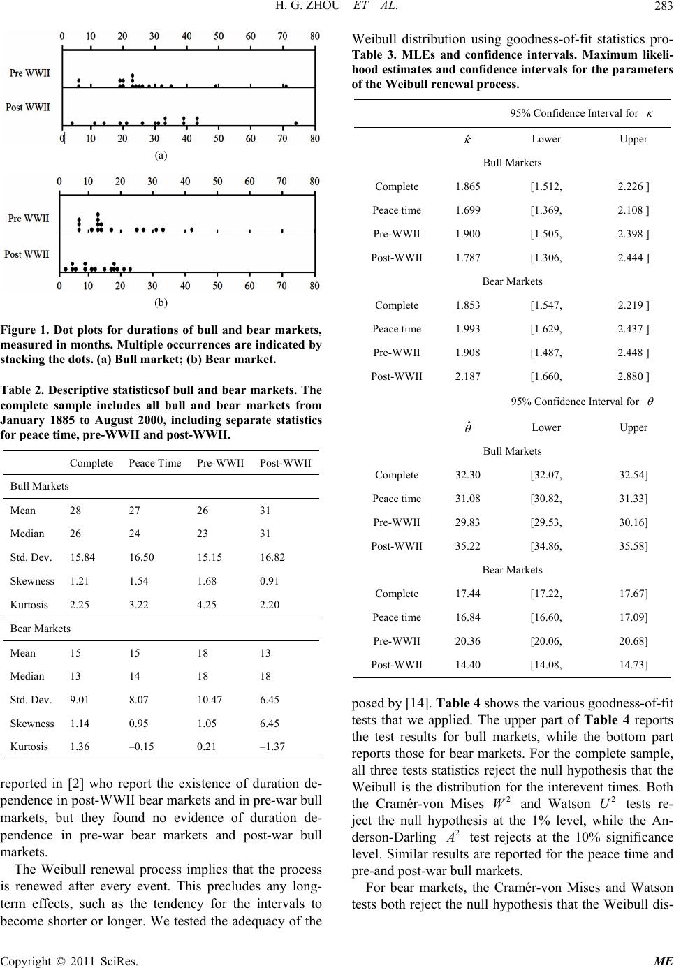

H. G. ZHOU ET AL. 283
(a)
(b)
Figure 1. Dot plots for durations of bull and bear markets,
measured in months. Multiple occurrences are indicated by
stacking the dots. (a) Bull market; (b) Bear market.
Table 2. Descriptive statisticsof bull and bear markets. The
complete sample includes all bull and bear markets from
January 1885 to August 2000, including separate statistics
for peace time, pre-WWII and post-WWII.
Complete Peace Time Pre-WWII Post-WWII
Bull Markets
Mean 28 27 26 31
Median 26 24 23 31
Std. Dev. 15.84 16.50 15.15 16.82
Skewness 1.21 1.54 1.68 0.91
Kurtosis 2.25 3.22 4.25 2.20
Bear Markets
Mean 15 15 18 13
Median 13 14 18 18
Std. Dev. 9.01 8.07 10.47 6.45
Skewness 1.14 0.95 1.05 6.45
Kurtosis 1.36 –0.15 0.21 –1.37
reported in [2] who report the existence of duration de-
pendence in post-WWII bear markets and in pre-war bull
markets, but they found no evidence of duration de-
pendence in pre-war bear markets and post-war bull
markets.
The Weibull renewal process implies that the process
is renewed after every event. This precludes any long-
term effects, such as the tendency for the intervals to
become shorter or longer. We tested the adequacy of the
Weibull distribution using goodness-of-fit statistics pro-
Table 3. MLEs and confidence intervals. Maximum likeli-
hood estimates and confidence intervals for the parameters
of the Weibull renewal pr oce ss.
95% Confidence Interval for

ˆ

Lower Upper
Bull Markets
Complete 1.865 [1.512, 2.226 ]
Peace time 1.699 [1.369, 2.108 ]
Pre-WWII 1.900 [1.505, 2.398 ]
Post-WWII 1.787 [1.306, 2.444 ]
Bear Markets
Complete 1.853 [1.547, 2.219 ]
Peace time 1. 993 [1.629, 2.437 ]
Pre-WWII 1.908 [1.487, 2.448 ]
Post-WWII 2.187 [1.660, 2.880 ]
95% Confidence Interval for

ˆ

Lower Upper
Bull Markets
Complete 32.30 [32.07, 32.54]
Peace time 31.08 [30.82, 31.33]
Pre-WWII 29.83 [29.53, 30.16]
Post-WWII 35.22 [34.86, 35.58]
Bear Markets
Complete 17.44 [17.22, 17.67]
Peace time 16.84 [16.60, 17.09]
Pre-WWII 20.36 [20.06, 20.68]
Post-WWII 14.40 [14.08, 14.73]
posed by [14]. Table 4 shows the various goo dn ess-of -f it
tests that we applied. The upper part of Table 4 reports
the test results for bull markets, while the bottom part
reports those for bear markets. For the complete sample,
all three tests statistics reject the null hypothesis that the
Weibull is the distribution for the interevent times. Both
the Cramér-von Mises2 and Watson2 tests re-
ject the null hypothesis at the 1% level, while the An-
derson-Darlin 2
W U
g
A
test rejects at the 10% significance
level. Similar results are reported for the peace time and
pre-and post-war bull m a rkets.
For bear markets, the Cramér-von Mises and Watson
tests both reject the null hypothesis that the Weibull dis-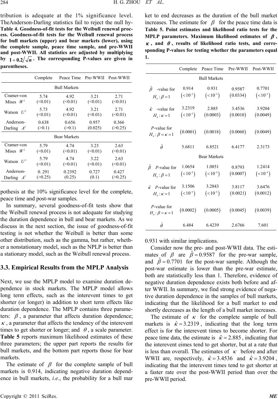

H. G. ZHOU ET AL. 284
tribution is adequate at the 1% significance level.
TheAnderson-Darling statistics fail to reject the null hy-
Table 4. Goodness-of-fit tests for the Weibull renewal proc-
ess. Goodness-of-fit tests for the Weibull renewal process
for bull markets (upper) and bear markets (lower), using
the complete sample, peace time sample, and pre-WWII
and post-WWII. All statistics are adjusted by multiplying
by 10.2 n. The corresponding P-values are given in
parentheses.
Complete Peace Time Pre-WWII Post-WWII
Bull Markets
Cramer-von
Mises
2
W5.74
(<0.01) 4.92 (<0.01) 3.21 (<0.01) 2.71 (<0.01)
Watson
2
U5.73
(<0.01) 4.92
(<0.01) 3.21 (<0.01) 2.71 (<0.01)
Anderson-
Darling 2
A
0.638
(>0.1) 0.656 (>0.1) 0.957 (0.025) 0.366 (>0.25)
Bear Markets
Cramer-von
Mises
2
W5.79
(<0.01) 4.74 (<0.01) 3.23 (<0.01) 2.63 (<0.01)
Watson
2
U5.79
(<0.01) 4.74 (<0.01) 3.22 (<0.01) 2.63 (<0.01)
Anderson-
Darling 2
A
0. 291
(>0.25) 0.2392 (0.25) 0.727 (0.1) 0.427 (>0.25)
pothesis at the 10% significance level for the complete,
peace time and post-war samples.
In summary, several goodness-of-fit tests show that
the Weibull renewal process is not adequate for stu dying
the duration dependence in bull and bear markets. As we
discuss in the next section, the issue of goodness-of-fit
testing is not whether the Weibull is better than some
other distribution, such as the gamma, but rather, wheth-
er a nonstationary model, such as the NPLP is better than
a stationary model, such as the Weibull renewal process.
3.3. Empirical Results from the MPLP Analysis
Next, we use the MPLP model to examine duration de-
pendence in stock markets. The MPLP model allows
long term effects, such as the interevent times to get
shorter (or longer) in addition to short term effects like
duration dependence. The MPLP contains three parame-
ters:

, a parameter that affects duration dependence;
, a parameter that affects the tendency of the interevent
times to get shorter or longer; and


, a scale parameter.
Table 5 reports maximum likelihood estimates of these
three parameters; the upper part reports the results for
bull markets, and the bottom part reports those for bear
markets.
The estimate of

for the complete sample of bull
markets is 0.914, indicating negative duration depend-
ence in bull markets, i.e., the probability for a bull mar
ket to end decreases as the duration of the bull market
increases. The estimate for

for the peace time data is
Table 5. Point estimates and likelihood ratio tests for the
MPLP parameters. Maximum likelihood estimates of

,

, and

, results of likelihood ratio tests, and corre-
sponding P-values for testing w hether the parameters equal
1.
CompletePeace Time Pre-WWII Post-WWII
Bull Markets
ˆ

-value for
0:1
 H

0.914


4
10 
0.931


4
10 
0.9587

0.0334
0.7701


4
10 
ˆ

-value for
0:1H


3.2319


4
10 
2.885


0.0003
3.4536

0.0010
3.9204


0.0049
P-value for
0:1H





0.0001


0.0018

0.0060


0.0049
ˆ

5.6811 6.8521 6.4177 2.3173
Bear Markets
ˆ

P-value for
0:1H


1.0654


4
10 
1.0851


4
10 
0.8793

0.0007
1.2414


4
10 
ˆ

P-value for
0:1H


3.1506


4
10 
3.2843


4
10 
3.8117
 0.0021
3.6476

 0.0012
P-value for
0:1H





0.0002


0.0005

0.0045


0.0039
ˆ

6.484 6.4239 2.6766 7.601
0.931 with similar im plications.
Consider now the pre- and post-WWII data. The esti-
mates of

are for the pre-war sample,
and for the post-war sample. Although the
post-war estimate is lower than the pre-war estimate,
both are statistically less than 1. Therefore, evidence of
negative duration dependence exists both before and af-
ter WWII. In summary, we find strong evidence of nega-
tive duration dependence in the samples of bull markets,
indicating that the likelihood for a bull market to end
shortly decreases as the length of a bull market increases.
ˆ0.95
 87
ˆ01
 0.77
The estimate of

for the complete sample of bull
markets is ˆ3.2319


, indicating that the long term
effect is for the interevent times to become shorter. For
peace time data, the estimate is , indicating that
the interevent eimes tend to get shorter, but at a rate that
is less than overall. The estimates of before and after
WWII are, respectively,
ˆ2.885
 

3.4536
ˆ

 and ˆ3.9204 

,
indicating that the interevent times tend to get shorter at
a faster rate over the post-WWII period than over the
pre-WW II perio d.

H. G. ZHOU ET AL.285
For the complete sample of bear markets, the estimate
of

is , indicating positive duration de-
pendence in bear markets. Therefore the probability that
a bear market ends increases with the length of the bear
market. This result is the opposite of that observed for
bull markets. There does seem to be a difference between
duration dependence in pre-war and post-war bear mar-
kets. For the pre-war data, the estimate is
(negative duration dependence) and for the post-war data,
the estimate is (positive duration depend-
ence). Both are significantly different from 1.
ˆ1.0654
 
ˆ
 
ˆ0.8793
 
1.2414
The estimates of exceed 3 for all cases considered
and all are significantly different from 1. These results
are similar to those for bull markets and indicate that the
cycles tend to become shorter over time. We also notice
that is higher for the peace time sample than for the
complete sample, indicating that wars slightly reduce the
resilience of bear markets to external shocks. There is
also a slight decrease in in the post-WWII sample
than in the pre-WWII sample, indicating that the intere-
vent times are getting shorter at a slower pace in the
post-WWII period. Based on the Frisch-Slutsky para-
digm, the lower indicates reduced resilience of bear
markets to external shocks in the post-WWII period than
in the pre-WWII perio d.

ˆ

ˆ

ˆ

Table 5 also gives the results of a number of hypothe-
sis tests. We test whether

or (or both simulta-
neously) are equal to 1. For these parameters, the value
of 1 is important; for


, the value 1

 is the bound-
ary between negative and positive duration dependence,
whereas for , the value  1


is the boundary be-
tween the cycles tending to get shorter or longer across
time. All of the hypothesis tests reject the null hypothesis
of the parameter being 1.
In summary, there is evidence of negative duration
dependence in all bull markets. There is evid ence of pos-
itive duration dependence in all bear markets except
those before WWII. Thus, bull markets tend to become
stronger and bear markets weaker as the cycle lengthens.
In regards to the long-term effect, the results show that
bull and bear markets tend to get progressively shorter,
but for bull markets, this trend has accelerated since
WWII, whereas for bear markets this trend has deceler-
ated since WWII. Finally, since the lengths of bull and
bear markets tend to get shorter over time, a stationary
model such as the Weibull renewal process, or any re-
newal process for that matter, is inadequate to model the
cycle times. A nonstationary model such as the MPLP is
needed.
4. Conclusions
Possible models for the stochastic point process that go-
verns financial cycles include the renewal process, the
NHPP, and the MPLP. The MPLP is a generalization of
both the renewal process and the NHPP in the sense that
if 1


, then the MPLP reduces to the NHPP, and if
1


, then the MPLP reduces to the Weibull renewal
process. If both 1


and , then the MPLP re-
duces to the homogeneo us Poi sso n pr ocess.
1  
Traditionally, the Weibull renewal process has been
applied as a model for business and financial cycles.
However, one of the assumptions implicitly made in the
Weibull renewal analysis seems dubious. The Weibull
renewal process also assumes that the underlying sto-
chastic process does not change across time. In other
words, a new market (i.e., a market that has just changed
from bull to bear, or vice-versa) is the same now as any
new market in the past. Considering that data come from
such a long period (1885 to 2000), this assumption ap-
pears unreasonable. A model is needed that can account
for both duration dependence and log term trends for
cycles to become shorter or longer. The MPLP, being a
compromise between the renewal process and the NHPP,
is such a model.
Results of goodness-of-fit tests reject the Weibull
process as a choice for modeling duration dependence of
bull and bear markets. The MPLP overcomes the short-
comings of the Weibull renewal process and is a more
powerful model for dependence in financial cycles.
The results indicate negative duration dependence in
all samples for bull markets and positive duration de-
pendence in complete, peace time, and post-WWII sam-
ples of bear markets. There is no evidence of structural
change after WWII in either bull or bear markets, with
the exception that bear markets seem to have negative
duration dependence before WWII and positive duration
dependence after. Results also indicate that both bull and
bear markets tend to get shorter over the long term, with
some evidence that the rates are different in the post-
WWII period and after excluding war time cycles.
5. Reference
[1] J. E. Payne and T. W. Zuehlke, “Duration Dependence in
Real Estate Investment Trusts,” Applied Financial Eco-
nomics, Vol. 16, No. 5, 2006, pp. 413-423.
doi:10.1080/09603100500391099
[2] S. J. Cochran and R. H. Defina, “Duration Dependence in
the US Stock Market Cycle: A Parametric Approach,”
Applied Financial Economics, Vol. 5, No. 5, 1995, pp.
27-37. doi:10.1080/758522757
[3] D. E. Sichel, “Business Cycle Duration Dependence: A
Parametric Approach,” The Review of Economics and
Statistics, Vol. 73, No. 2, 1991, pp. 254-260.
doi:10.2307/2109515
[4] H. Zhou and S. E. Rigdon, “Duration Dependence in U.S.

H. G. ZHOU ET AL. 286
Business Cycles: An Analysis Using the Modulated
Power Law Process,” Journal of Economics and Finance,
Vol. 32, No. 1, 2008, pp. 25-34.
doi:10.1007/s12197-007-9005-3
[5] M. Berman, “Inhomogeneous and Modulated Gamma
Processes,” Biometrika, Vol. 68, No. 1, 1982, pp. 142-
152.
[6] M. J. Lakey and S. E. Rigdon, “The Modulated Power
Law Process,” Proceedings of the 45th Annual Quality
Congress, Milwaukee, 20-22 May 1991, pp. 559-563.
[7] S. E. Black and S. E. Rigdon, “Statistical Inference for a
Modulated Power Law Process,” Journal of Quality
Technology, Vol. 28, No. 1, 1996, pp. 81-90.
[8] R. Frisch, “Propagation and Impulse Problems in Dy-
namic Economics,” Economic Essays in Honor of Gustav
Cassel, Allen and Unwin, London, 1933, pp. 171-173,
181-190, 197-203.
[9] E. Slutsky, “The Summation of Random Causes as the
Source of Cyclic Processes,” Econometrica, Vol. 5, No. 2,
1937, pp. 105-146. doi:10.2307/1907241
[10] S. Chatterjee, “From Cycles to Shocks: Progress in Busi-
ness-Cycle Theory,” 2000.
http://www.phil.frb.org/files/br/brma00sc.pdf
[11] B. S. Bernanke, M. Gertler and S. Gilchrist, “The Finan-
cial Accelerator in a Quantitative Business Cycle Frame-
work,” Review of Economics and Statistics, Vol. 78, No.
1, 1996, pp. 1-15.
[12] C. Nolan and C. Thoenissen, “Financial Shocks and the
US Business Cycle,” Journal of Monetary Economics,
Vol. 56, No. 4, 2009, pp. 596-604.
doi:10.1016/j.jmoneco.2009.03.007
[13] A. R. Pagan and K. A. Sossounov, “A Simple Framework
for Analysing Bull and Bear Markets,” Journal of Ap-
plied Econometrics, Vol. 18, No. 1, 2003, pp. 23-46.
doi:10.1002/jae.664
[14] M. A. Stephens, “Tests Based on EDF Statistics,” In: R.
B. D’Agostino and M. A. Stephens, Eds., Goodness-of-
-Fit Techniques, Marcel Dekker, New York, 1986, pp.
97-193.