Atmospheric and Climate Sciences, 2011, 1, 120-133
doi:10.4236/acs.2011.13014 Published Online July 2011 (http://www.scirp.org/journal/acs)
On the Fractal Mechanism of Interrelation between the
Genesis, Size and Composition of Atmospheric Particulate
Matters in Different Regions of the Earth
Vitaliy D. Rusov1*, Radomir Ilić2#, Radojko Jaćimović2, Vladimir N. Pavlovich3,
Yuriy A. Bondarchuk1, Vladimir N. Vaschenko4, Tatiana N. Zelentsova1, Margarita E. Beglaryan1,
Elena P. Linnik1, Vladimir P. Smolyar1, Sergey I. Kosenko1, Alla A. Gudyma4
1Odessa National Polytechnic University, Odessa, Ukraine
2Josef Stefan Institute, Ljubljana, Slovenia
3Institute for Nuclear Research, Kyiv, Ukraine
4State Ecological Academy for Postgraduate Education and Management, Kyiv, Ukraine
E-Mails:
Abstract
Experimental data from the National Air Surveillance Network of Japan from 1974 to 1996 and from inde-
pendent measurements performed simultaneously in the regions of Ljubljana (Slovenia), Odessa (Ukraine)
and the Ukrainian “Academician Vernadsky” Antarctic station (64˚15'W; 65˚15'S), where the air elemental
composition was determined by the standard method of atmospheric particulate matter (PM) collection on
nucleopore filters and subsequent neutron activation analysis, were analyzed. Comparative analysis of dif-
ferent pairs of atmospheric PM element concentration data sets, measured in different regions of the Earth,
revealed a stable linear (on a logarithmic scale) correlation, showing a power law increase of every atmos-
pheric PM element mass and simultaneously the cause of this increase—fractal nature of atmospheric PM
genesis. Within the framework of multifractal geometry we show that the mass (volume) of atmospheric PM
elemental components has a log normal distribution, which on a logarithmic scale with respect to the random
variable (elemental component mass) is identical to normal distribution. This means that the parameters of
two-dimensional normal distribution with respect to corresponding atmospheric PM-multifractal elemental
components measured in different regions, are a priory connected by equations of direct and inverse linear
regression, and the experimental manifestation of this fact is the linear correlation between the concentra-
tions of the same elemental components in different sets of experimental atmospheric PM data.
Keywords: Atmospheric Aerosols, Multifractal, Neutron activation analysis, South Pole, Ukrainian Antarctic
station
1. Introduction
Analysis of the concentrations of elements characteristics
of the terrestrial crust, anthropogenic emissions and marine
elements used in monitoring of the levels of atmospheric
aerosol contamination indicates that these levels at the two
extremes of: 1) the Antarctic (South Pole [1]), and 2) the
global constituent of atmospheric contamination measured
at continental background stations [2] display similar pat-
terns. A distinction between them is, however, evident and
consists in that the mean element concentrations in the at-
mosphere over continental background stations (СCB) lo-
cated in different regions of the Earth exceed the corre-
sponding concentrations at the South Pole (СSP) by some
20 - 1000 times.
Comparing the concentrations of a given element i in
atmospheric aerosol from samples {CSP,i} and {CCB,i}, it
became evident that the dependence of the mean concen-
trations of any particular element from the sample {CSP,i}
or {CCB,i} on a logarithmic scale is described by a linear
one, with good precision for any of the elements from a
given pair of sampling station:
In In
ii
CBCB SPCB SPSP
Ca bC

 (1)
1
CB SP
b (2)
#Deceased.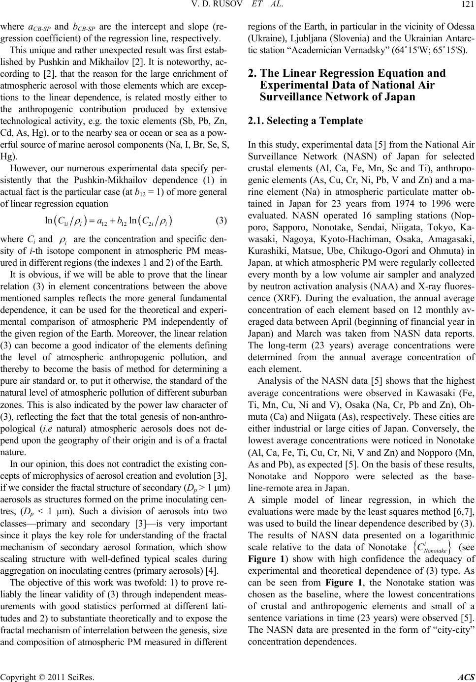

V. D. RUSOV ET AL.121
where аCB-SP and bCB-SP are the intercept and slope (re-
gression coefficient) of the regression line, respectively.
This unique and rather unexpected result was first estab-
lished by Pushkin and Mikhailov [2]. It is noteworthy, ac-
cording to [2], that the reason for the large enrichment of
atmospheric aerosol with those elements which are excep-
tions to the linear dependence, is related mostly either to
the anthropogenic contribution produced by extensive
technological activity, e.g. the toxic elements (Sb, Pb, Zn,
Cd, As, Hg), or to the nearby sea or ocean or sea as a pow-
erful source of marine aerosol components (Na, I, Br, Se, S,
Hg).
However, our numerous experimental data specify per-
sistently that the Pushkin-Mikhailov dependence (1) in
actual fact is the particular case (at b12 = 1) of more general
of linear regression equation
 
112122
ln ln
ii ii
CabC


  (3)
where Сi and i

are the concentration and specific den-
sity of i-th isotope component in atmospheric PM meas-
ured in different regions (the indexes 1 and 2) of the Earth.
It is obvious, if we will be able to prove that the linear
relation (3) in element concentrations between the above
mentioned samples reflects the more general fundamental
dependence, it can be used for the theoretical and experi-
mental comparison of atmospheric PM independently of
the given region of the Earth. Moreover, the linear relation
(3) can become a good indicator of the elements defining
the level of atmospheric anthropogenic pollution, and
thereby to become the basis of method for determining a
pure air standard or, to put it otherwise, the standard of the
natural level of atmospheric pollution of different suburban
zones. This is also indicated by the power law character of
(3), reflecting the fact that the total genesis of non-anthro-
pological (i.e natural) atmospheric aerosols does not de-
pend upon the geography of their origin and is of a fractal
nature.
In our opinion, this does not contradict the existing con-
cepts of microphysics of aerosol creation and evolution [3],
if we consider the fractal structure of secondary (Dp > 1 μm)
aerosols as structures formed on the prime inoculating cen-
tres, (Dp < 1 μm). Such a division of aerosols into two
classes—primary and secondary [3]—is very important
since it plays the key role for understanding of the fractal
mechanism of secondary aerosol formation, which show
scaling structure with well-defined typical scales during
aggregation on inoculating centres (primary aerosols) [4].
The objective of this work was twofold: 1) to prove re-
liably the linear validity of (3) through independent meas-
urements with good statistics performed at different lati-
tudes and 2) to substantiate theoretically and to expose the
fractal mechanism of interrelation between the genesis, size
and composition of atmospheric PM measured in different
regions of the Earth, in particular in the vicinity of Odessa
(Ukraine), Ljubljana (Slovenia) and the Ukrainian Antarc-
tic station “Academician Vernadsky” (64˚15'W; 65˚15'S).
2. The Linear Regression Equation and
Experimental Data of National Air
Surveillance Network of Japan
2.1. Selecting a Template
In this study, experimental data [5] from the National Air
Surveillance Network (NASN) of Japan for selected
crustal elements (Al, Ca, Fe, Mn, Sc and Ti), anthropo-
genic elements (As, Cu, Cr, Ni, Pb, V and Zn) and a ma-
rine element (Na) in atmospheric particulate matter ob-
tained in Japan for 23 years from 1974 to 1996 were
evaluated. NASN operated 16 sampling stations (Nop-
poro, Sapporo, Nonotake, Sendai, Niigata, Tokyo, Ka-
wasaki, Nagoya, Kyoto-Hachiman, Osaka, Amagasaki,
Kurashiki, Matsue, Ube, Chikugo-Ogori and Ohmuta) in
Japan, at which atmospheric PM were regularly collected
every month by a low volume air sampler and analyzed
by neutron activation analysis (NAA) and X-ray fluores-
cence (XRF). During the evaluation, the annual average
concentration of each element based on 12 monthly av-
eraged data between April (beginning of financial year in
Japan) and March was taken from NASN data reports.
The long-term (23 years) average concentrations were
determined from the annual average concentration of
each element.
Analysis of the NASN data [5] shows that the highest
average concentrations were observed in Kawasaki (Fe,
Ti, Mn, Cu, Ni and V), Osaka (Na, Cr, Pb and Zn), Oh-
muta (Ca) and Niigata (As), respectively. These cities are
either industrial or large cities of Japan. Conversely, the
lowest average concentrations were noticed in Nonotake
(Al, Ca, Fe, Ti, Cu, Cr, Ni, V and Zn) and Nopporo (Mn,
As and Pb), as expected [5]. On the basis of these results,
Nonotake and Nopporo were selected as the base-
line-remote area in Japan.
A simple model of linear regression, in which the
evaluations were made by the least squares method [6,7],
was used to build the linear dependence described by (3).
The results of NASN data presented on a logarithmic
scale relative to the data of Nonotake

i
N
onotake
C (see
Figure 1) show with high confidence the adequacy of
experimental and theoretical dependence of (3) type. As
can be seen from Figure 1, the Nonotake station was
chosen as the baseline, where the lowest concentrations
of crustal and anthropogenic elements and small of a
sentence variations in time (23 years) were observed [5].
The NASN data are presented in the form of “city-city”
concentration dependences.

V. D. RUSOV ET AL. 122
Analysis of concentration data for Japanese city at-
mospheric PM unambiguously shows that the i-th ele-
ment mass in atmospheric PM grows by power low,
proving the assumption [4,8-10] about the fractal nature
of atmospheric PM genesis.
3. The Linear Regression Equation and the
Composition of Atmospheric Aerosols in
Different Regions of the Earth
It is evident that in order to generalize the results from
NASN data processing more widely, the validity of (3)
should be checked on the basis of atmospheric aerosol
studies in performed independent experiments at differ-
ent latitudes. For this reason such studies were performed
in the regions of Odessa (Ukraine), Ljubljana (Slovenia)
and the Ukrainian Academecian Vernadsky Antarctic
station (64˚15'W; 65˚15'S). The determination of the
element composition of the atmospheric air in these ex-
periments was performed by the traditional method based
on collection of atmospheric aerosol particles on nu-
cleopore filters with subsequent use of k0-instrumental
neutron activation analysis. Regression analysis was used
for processing of the experimental data.
3.1. Experimental
3.1.1. Collection of Atmospheric Aerosol Particles
on Nucleopore Filters
For collection of atmospheric aerosolparticles on filters,
a device of the PM10 type was used with the Gent
Stacked Filter Unit (SFU) interface [11,12]. The main
part of this device is a flow-chamber containing an im-
pactor, the throughput capacity of which is equivalent to
the action of a filter with an aerodynamic pore diameter
of 10 μm and a 50% aerosol particle collection efficiency
based on mass, and an SFU interface designed by the
Norwegian Institute for Air Research (NILU) and con-
taining two filters (Nucleopore) each 47 mm in diameter,
the first filter with a pore diameter of 8 μm and the sec-

V. D. RUSOV ET AL.123
Figure 1. Relation between annual concentrations of elements in atmospheric particulate matter over Japan and the same
data obtained in the region of Nonotake (data from NASN of Japan [5]). In some cases (see text) the concentration of anthro-
pogenic element Cr was excluded from the data. The underlined cities are large industrial centres in the Japan [5].
Figure 2. Schematic representation of the flow-chamber of
the PM10 type device for air sampling.
ond filter with 0.4 μm pore diameter. It was experimen-
tally found [12] that such geometry (Figure 2) results in
an aerosol collection efficiency of the first filter of ap-
proximately 50%, whereas for the second filter this value
was close to 100% [12]. More detailed results of thor-
ough testing of a similar device can be found in [12]. The
template is used to format your paper and style the text.
3.1.2. K0-Instrumental Neutron Activation
Analysis
Airborne particulate matter (APM) loaded filters were
pelleted with a manual press to a pellet of 5 mm di-
ameter and each packed in a polyethylene ampoule,
together with an Al-0.1% Au IRMM-530 disk 6 mm in
diameter and 0.2 mm thickness and irradiated for short
irradiations (2 - 5 min) in the pneumatic tube (PT) of
the 250 kW TRIGA Mark II reactor of the J. Stefan
Institute at a thermal neutron flux of 3.5·1012 cm–2·s–1,
and for longer irradiations in the carousel facility (CF)
at a thermal neutron flux of 1.1·1012 cm–2·s–1 (irradia-
tion time for each sample about 18 - 20 h). After irra-
diation, the sample and standard were transferred to
clean 5 mL polyethylene mini scintillation vial for
gamma ray measurement.
To determine the ratio of the thermal to epithermal
neutron flux (f) and the parameter

, which charac-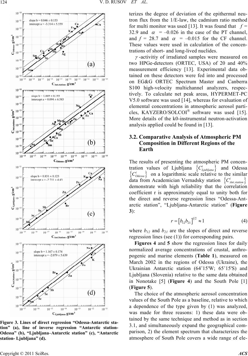

V. D. RUSOV ET AL. 124
Figure 3. Lines of direct regression “Odessa-Antarctic sta-
tion” (a), line of inverse regression “Antarctic station-
Odessa” (b), “Ljubljana–Antarctic station” (c), “Antarctic
station- Ljubljana” (d).
terizes the degree of deviation of the epithermal neu-
tron flux from the 1/E-law, the cadmium ratio method
for multi monitor was used [13]. It was found that
f
=
32.9 and

= –0.026 in the case of the РТ channel,
and f = 28.7 and

= –0.015 for the CF channel.
These values were used in calculation of the concen-
trations of short- and long-lived nuclides.

-activitiy of irradiated samples were measured on
two HPGe-detectors (ORTEC, USA) of 20 and 40%
measurement efficiency [13]. Experimental data ob-
tained on these detectors were fed into and processed
on EG&G ORTEC Spectrum Master and Canberra
S100 high-velocity multichannel analyzers, respec-
tively. To calculate net peak areas, HYPERMET-PC
V5.0 software was used [14], whereas for evaluation of
elemental concentrations in atmospheric aerosol parti-
cles, KAYZERO/SOLCOI software was used [15].
More details of the k0-instrumental neutron-activation
analysis applied could be found in [13].
3.2. Comparative Analysis of Atmospheric PM
Composition in Different Regions of the
Earth
The results of presenting the atmospheric PM concen-
tration values of Ljubljana

i
L
jubljana
C and Odessa


i
Odessa
C on a logarithmic scale relative to the similar
data from Academician Vernadsky station


.
i
Ant station
C
demonstrate with high reliability that the correlation
coefficient r is approximately equal to unity both for
the direct and reverse regression lines “Odessa-Ant-
arctic station”, “Ljubljana-Antarctic station” (Figure
3):

12
12 211rbb

 (4)
where b12 and b21 are the slopes of direct and reverse
regression lines (see (1)) for corresponding pairs.
Figures 4 and 5 show the regression lines for daily
normalized average concentrations of crustal, anthro-
pogenic and marine elements (Table 1), measured on
March 2002 in the regions of Odessa (Ukraine), the
Ukrainian Antarctic station (64˚15'W; 65˚15'S) and
Ljubljana (Slovenia) relative to the same data obtained
in Nonotake [5] (Figure 4) and the South Pole [1]
(Figure 5).
The choice of the atmospheric aerosol concentration
values of the South Pole as a baseline, relative to which
a dependence of the type given by (1) was analyzed,
was made for three reasons: 1) these data were ob-
tained by the same technique and method as in section
3.1, and simultaneously expand the geographical com-
parison, 2) the element spectrum that characterizes the
atmosphere of South Pole covers a wide range of ele-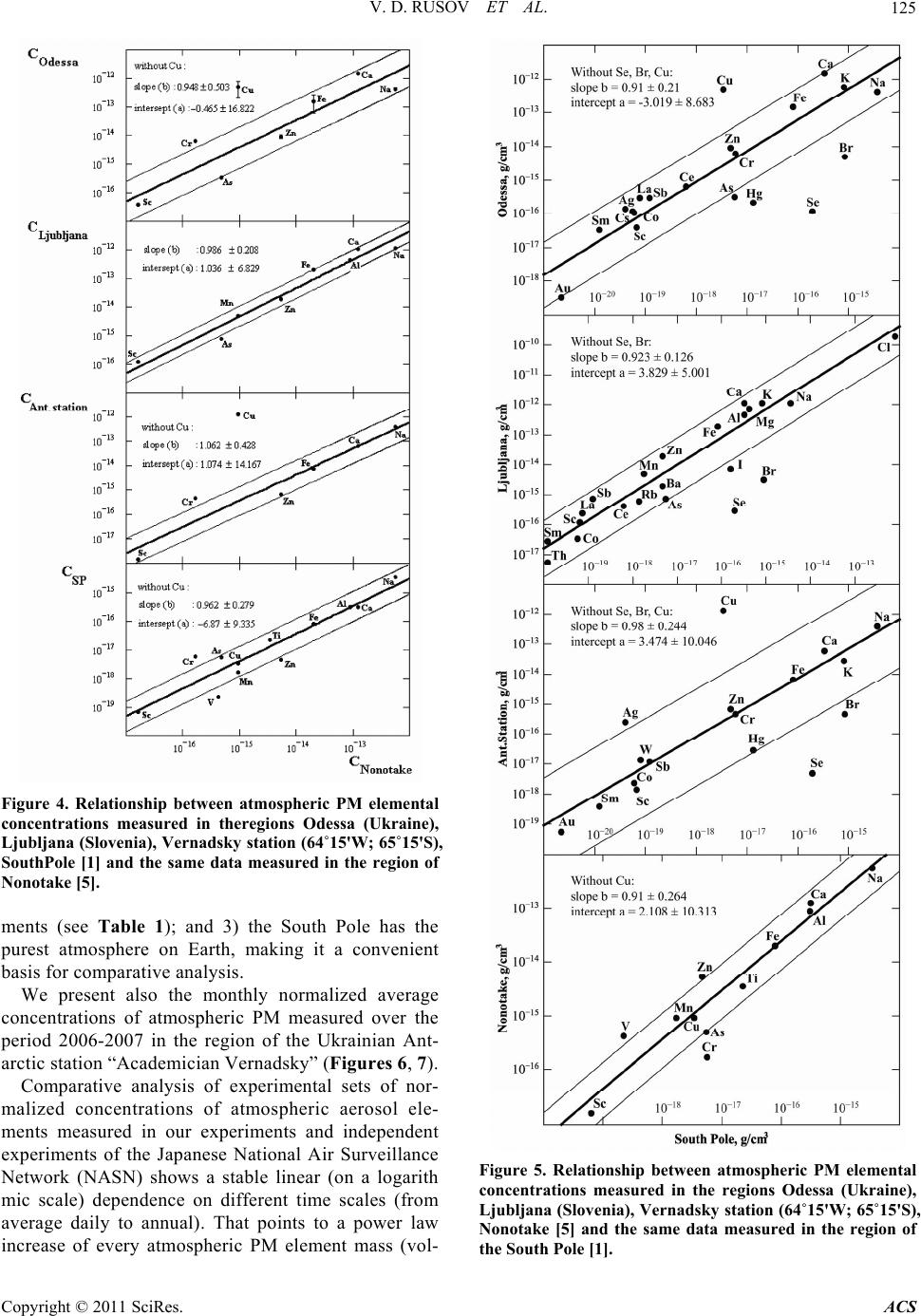

V. D. RUSOV ET AL.125
Figure 4. Relationship between atmospheric PM elemental
concentrations measured in theregions Odessa (Ukraine),
Ljubljana (Slovenia), Vernadsky station (64˚15'W; 65˚15'S),
SouthPole [1] and the same data measured in the region of
Nonotake [5].
ments (see Table 1); and 3) the South Pole has the
purest atmosphere on Earth, making it a convenient
basis for comparative analysis.
We present also the monthly normalized average
concentrations of atmospheric PM measured over the
period 2006-2007 in the region of the Ukrainian Ant-
arctic station “Academician Vernadsky” (Figures 6, 7).
Comparative analysis of experimental sets of nor-
malized concentrations of atmospheric aerosol ele-
ments measured in our experiments and independent
experiments of the Japanese National Air Surveillance
Network (NASN) shows a stable linear (on a logarith
mic scale) dependence on different time scales (from
average daily to annual). That points to a power law
increase of every atmospheric PM element mass (vol-
Figure 5. Relationship between atmospheric PM elemental
concentrations measured in the regions Odessa (Ukraine),
Ljubljana (Slovenia), Vernadsky station (64˚15'W; 65˚15'S),
Nonotake [5] and the same data measured in the region of
the South Pole [1].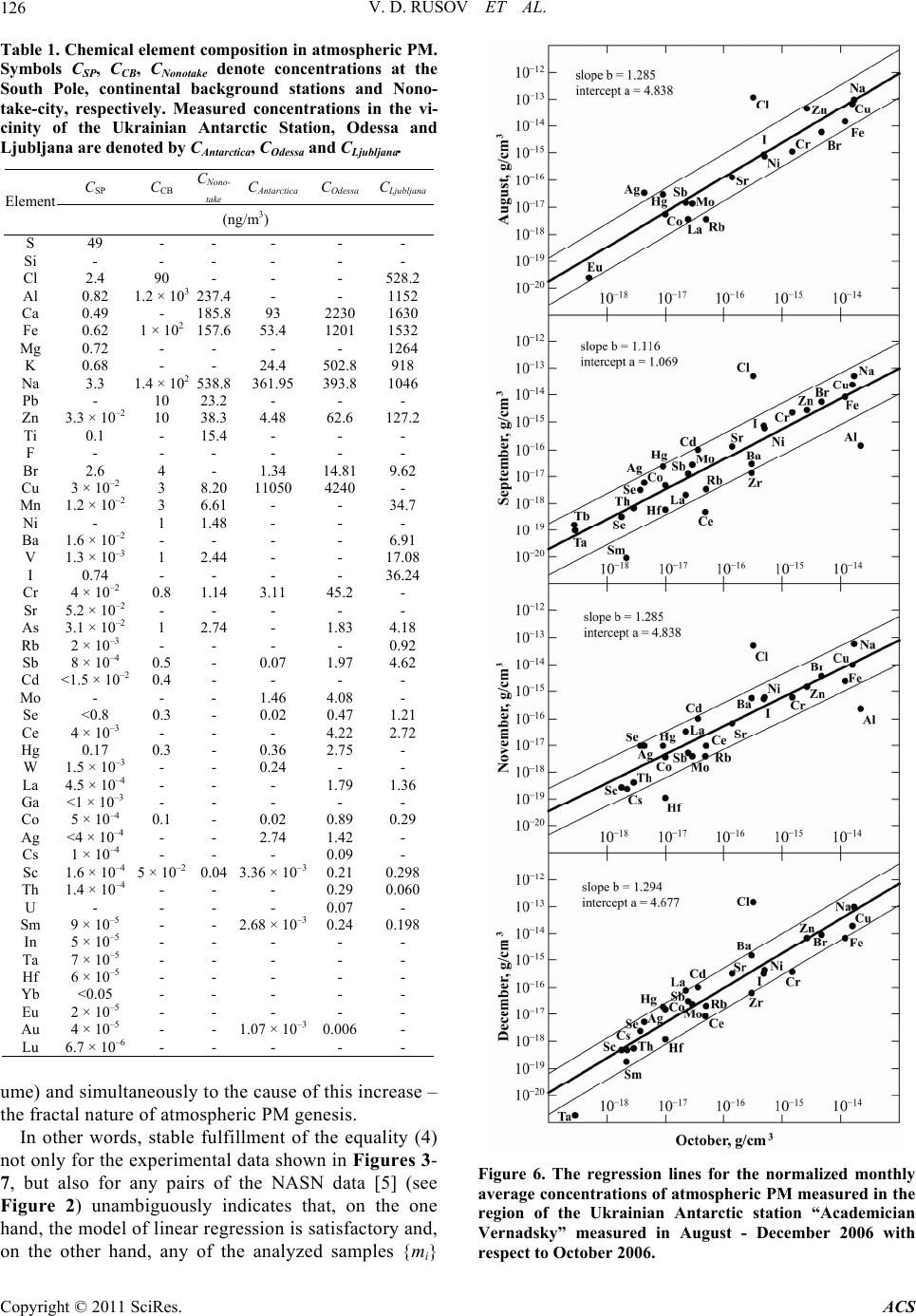

V. D. RUSOV ET AL. 126
Table 1. Chemical element composition in atmospheric PM.
Symbols CSP, CCB, CNonotake denote concentrations at the
South Pole, continental background stations and Nono-
take-city, respectively. Measured concentrations in the vi-
cinity of the Ukrainian Antarctic Station, Odessa and
Ljubljana are denoted by CAntarctica, COdessa and CLjubljana.
СSP СCB
CNono-
take САntarctica СОdessa CLjubljana
Element
(ng/m3)
S 49 - - - - -
Si - - - - - -
Cl 2.4 90 - - - 528.2
Al 0.82 1.2 × 103 237.4- - 1152
Ca 0.49 - 185.893 2230 1630
Fe 0.62 1 × 102 157.653.4 1201 1532
Mg 0.72 - - - - 1264
K 0.68 - - 24.4 502.8 918
Na 3.3 1.4 × 102 538.8361.95 393.8 1046
Pb - 10 23.2- - -
Zn 3.3 × 10–2 10 38.34.48 62.6 127.2
Ti 0.1 - 15.4- - -
F - - - - - -
Br 2.6 4 - 1.34 14.81 9.62
Cu 3 × 10–2 3 8.2011050 4240 -
Mn 1.2 × 10–2 3 6.61- - 34.7
Ni - 1 1.48- - -
Ba 1.6 × 10–2 - - - - 6.91
V 1.3 × 10–3 1 2.44- - 17.08
I 0.74 - - - - 36.24
Cr 4 × 10–2 0.8 1.143.11 45.2 -
Sr 5.2 × 10–2 - - - - -
As 3.1 × 10–2 1 2.74- 1.83 4.18
Rb 2 × 10–3 - - - - 0.92
Sb 8 × 10–4 0.5 - 0.07 1.97 4.62
Cd <1.5 × 10–2 0.4 - - - -
Mo - - - 1.46 4.08 -
Se <0.8 0.3 - 0.02 0.47 1.21
Ce 4 × 10–3 - - - 4.22 2.72
Hg 0.17 0.3 - 0.36 2.75 -
W 1.5 × 10–3 - - 0.24 - -
La 4.5 × 10–4 - - - 1.79 1.36
Ga <1 × 10–3 - - - - -
Co 5 × 10–4 0.1 - 0.02 0.89 0.29
Ag <4 × 10–4 - - 2.74 1.42 -
Cs 1 × 10–4 - - - 0.09 -
Sc 1.6 × 10–4 5 × 10–2 0.043.36 × 10–3 0.21 0.298
Th 1.4 × 10–4 - - - 0.29 0.060
U - - - - 0.07 -
Sm 9 × 10–5 - - 2.68 × 10–3 0.24 0.198
In 5 × 10–5 - - - - -
Ta 7 × 10–5 - - - - -
Hf 6 × 10–5 - - - - -
Yb <0.05 - - - - -
Eu 2 × 10–5 - - - - -
Au 4 × 10–5 - - 1.07 × 10–3 0.006 -
Lu 6.7 × 10–6 - - - - -
ume) and simultaneously to the cause of this increase –
the fractal nature of atmospheric PM genesis.
In other words, stable fulfillment of the equality (4)
not only for the experimental data shown in Figures 3-
7, but also for any pairs of the NASN data [5] (see
Figure 2) unambiguously indicates that, on the one
hand, the model of linear regression is satisfactory and,
on the other hand, any of the analyzed samples mi
Figure 6. The regression lines for the normalized monthly
average concentrations of atmospheric PM measured in the
region of the Ukrainian Antarctic station “Academician
Vernadsky” measured in August - December 2006 with
respect to October 2006.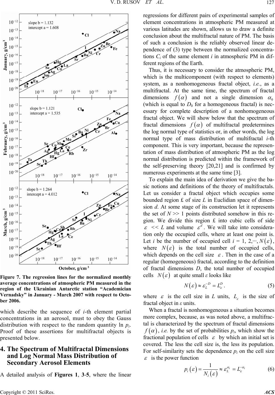

V. D. RUSOV ET AL.127
Figure 7. The regression lines for the normalized monthly
average concentrations of atmospheric PM measured in the
region of the Ukrainian Antarctic station “Academician
Vernadsky” in January - March 2007 with respect to Octo-
ber 2006.
which describe the sequence of i-th element partial
concentrations in an aerosol, must to obey the Gauss
distribution with respect to the random quantity ln pi.
Proof of these assertions for multifractal objects is
presented below.
4. The Spectrum of Multifractal Dimensions
and Log Normal Mass Distribution of
Secondary Aerosol Elements
A detailed analysis of Figures 1, 3-5, where the linear
regressions for different pairs of experimental samples of
element concentrations in atmospheric PM measured at
various latitudes are shown, allows us to draw a definite
conclusion about the multifractal nature of PM. The basis
of such a conclusion is the reliably observed linear de-
pendence of (3) type between the normalized concentra-
tions Сi of the same element i in atmospheric PM in dif-
ferent regions of the Earth.
Thus, it is necessary to consider the atmospheric PM,
which is the multicomponent (with respect to elements)
system, as a nonhomogeneous fractal object, i.e., as a
multifractal. At the same time, the spectrum of fractal
dimensions


f

and not a single dimension 0

(which is equal to D0 for a homogeneous fractal) is nec-
essary for complete description of a nonhomogeneous
fractal object. We will show below that the spectrum of
fractal dimensions


f

of multifractal predetermines
the log normal type of statistics or, in other words, the log
normal type of mass distribution of multifractal i-th
component. This is very important, because the represen-
tation of mass distribution of atmospheric PM as the log
normal distribution is predicted within the framework of
the self-preserving theory [20,21] and is confirmed by
numerous experiments at the same time [3].
To explain the main idea of derivation we give the ba-
sic notions and definitions of the theory of multifractals.
Let us consider a fractal object which occupies some
bounded region £ of size L in Euclidian space of dimen-
sion d. At some stage of its construction let it represents
the set of N >> 1 points distributed somehow in this re-
gion. We divide this region £ into cubic cells of side

<< L and volume d

. We will take into considera-
tion only the occupied cells, where at least one point is.
Let i be the number of occupied cell i = 1, 2,···,


N

,
where


N

is the total number of occupied cells,
which depends on the cell size

. Then in the case of a
regular (homogeneous) fractal, according to the definition
of fractal dimensions D, the total number of occupied
cells


N

at quite small ε looks like


D
D
L
NL




. (5)
where

is the cell size in L units, L

is the size of
fractal object in ε units.
When a fractal is nonhomogeneous a situation becomes
more complex, because, as was noted above, a multifrac-
tal is characterized by the spectrum of fractal dimensions


f

, i.e. by the set of probabilities pi, which show the
fractional population of cells

by which an initial set is
covered. The less the cell size is, the less its population.
For self-similarity sets the dependence pi on the cell size

is the power function
 
1i
iL
i
pL
N
i






 (6)

V. D. RUSOV ET AL. 128
where i

is a certain exponent which, generally speak-
ing, is different for the different cells i. It is obvious, that
for a regular (homogeneous) fractal all the indexes i

in
(6) are identical and equal to the fractal dimension D.
We now pass on to probability distribution of the dif-
ferent values i

Let

nd

 is the probability what
αi is in the interval


, +d

 . In other words,

nd

 is the relative number of the cells i, which
have the same measure pi as i

in the interval


, +d

 . According to (5), this number is propor-
tional to the total number of cells

D
L
N



 for a
monofractal, since all of i

are identical and equal to
the fractal dimension D.
However, this is not true for a multifractal. The differ-
ent values of i

occur with probability characterized by
the different (depending on

) values of the exponent

f

, and this probability inherently corresponds to a
spectrum of fractal dimensions of the homogeneous sub-
sets £

of initial set £:


f
L
n



. (7)
Thus, from here a term “multifractal” becomes clear. It
can be understood as a hierarchical joining of the differ-
ent but homogeneous fractal subsets £

of initial set £,
and each of these subsets has the own value of fractal
dimension


f

.
Now we show how the function

f

predetermines
the log normal kind of mass (volume) distribution of the
multifractal i-th component. To ease further description
we represent expression (8) in the following equivalent
form:



exp lnnfL

 
 
. (8)
It is not hard to show [19] that the single-mode func-
tion


f

can be approximated by a parabola near its
maximum at the value 0

.
 
2
0
fD  

0
(9)
where the curvature of parabola
0
00 0
() 1
222() q
f
DD




 



(10)
is determined by the second derivative of function


f

at a point 0

. Due to a convexity of the function


f

it is obvious, that the magnitude in square brackets must
be always positive. The fact, that the last summand 0q
D



in these brackets is numerically small and it can be ne-
glected, will be grounded below.
At the large L

the distribution

n

(8) with an
allowance for (9) takes on the form

2
0
0
00
ln
()~exp ln4()
L
nDL D










. (11)
Then, taking into account (5), we obtain from (11) the
distribution function of random variable pi




0
0
2
0
0
exp
~ln
1ln ln
4ln 1
Di
i
D
Nnp
pp
pN







(12)
which with consideration of normalization takes on the
final form


2
2
2
11
exp 2
2
1
expln
2
i
i
Pp
p











 




(13)
where
0
2
0
0
ln 1
1n , =2
N
pp   (14)
This is the so-called log normal (relative) mass pi dis-
tribution. It is possible to present the first moments of
such a kind of distribution for random variable pi in the
following form:

00
0
23 223
0
3
exp 1
2
D
Ds
ppN




 

 L
(15)
 
 


00 00
22
22 322
varexp2exp 4exp 3
1
DD
p
LL


 



 



(16)
At the same time, it is easy to show that the distribu-
tion (13) for the random variable ln pi has the classical
Gaussian form


2
2
2
1
1n
2
1
exp1n 1n
2
Pp
pp













(17)
where the first moments of this distribution for the ran-
dom variable ln pi look like



2
00
1n 21npD L

    (18)



2
00
var1n 21npaD L

   (19)
Thus, according to the known theorem of multidimen-
sional normal distribution shape [22], a normal law of
plane distribution for the two-dimensional random vari-
able (p1i, p2i) will be written down as



12 2
12
22
2
1
1n ,1n
21
1
exp 2
21
ii
pp p
r
uv ruv
r
 







 





(20)

V. D. RUSOV ET AL.129
where
112 2
12
1n 1n 1n 1n
, (21)
iiii
pp pp
v 


= cov(ln p1i, ln p2i)/σ1 σ2 is the correlation coefficient
between ln p1i and ln p2i.
, by virtue of well-known linear correlation theo-
rem [6,22] it is easy to show that ln p1i and ln p2i are con-
nected by the linear correlation dependen
two-dimensional random variable (ln p1i, ln p2i) is nor-
m
r
Then
ce, if the
ally distributed. This means that the parameters of
two-dimensional normal distribution of the random val-
ues p1i and p2i for the i-th component in one aerosol parti-
cle, which are measured in different regions of the Earth
(the indexes 1 and 2), are connected by the equations of
direct linear regression:
1
112 2
2
1n 1n 1n 1n
i
iii i
i
pprp p



 

 (21)
and inverse linear regression
2
22
1n 1n i
ii
pp

11
1
1n 1n
ii
i
r pp


 

 (22)
where I = 1,···,Np is the component number.
Taking into consideration that we measure experimen-
i of the i-th component in
the unit volume of atmosphere, the partial concentration
mi of the i-th component in one aerosol particle
in different regions of the Earth (the indexes 1 and 2)
tally the total concentration С
measured
looks lik
111122
,
iii i
mCnmCn (23)
where n1 and n2 are the number of inoculating centers,
whose role play the primary aerosols (Dp < 1 μm).
Here it is necessary to make important digression con-
cerning the choice of quantitative measure for description
of fractal structures. According to Feder [18]
tion of appropriate probabilities correspo
ure of
pr
, determina-
nding to the
chosen measure is the main difficulty. In other words, if
choice of measure determines the search proced
obabilities pi, which describe the increment of the
chosen measure for given level of resolution

, then the
probabilities themselves predetermine, in its turn, the
proper method of their measurement. So, general strategy
of quantitative description of fractal objects, in general
case, should contain the following direct or reverse pro-
cedure: the choice of measure—the set of appropriate
probabilities—the measuring method of these probabili-
ties.
We choose the reverse procedure. So long as in the
present work the averaged masses of elemental compo-
nents of atmospheric PM-multifractal are measured, the
geometrical probabilities, which can be constructed by
experimental data for some fixed

, have the practically
unambiguous form:

//
//
iii
i
ii ii
ii
mi C
p constmC





 


(24)
where ρi is the specific gravity of the i-th component of
secondary aerosol.
Since the random nature of atmospheric PM formation
is a priori determined by the random process
component diffusion-limited aggregation (DLA),
the so-called harmonic measure [18] to describe quantita-
volution of possible growth of cluster
PM
ster. Both these magnitudes, Np and N,
ch
of multi-
we used
tively a stochastic surface inhomogeneity or, more pre-
cisely, to study an e
diameter.
In practice, a harmonic measure is estimated in the fol-
lowing way. Because the perimeter of clusters, which
form due to DLA, is proportional to their mass, the num-
ber of knots Np on the perimeter, i.e., the number of pos-
sible growing-points, is proportional to the number of
cells N in a clu
ange according to the power law (5) depending on the
cluster diameter L. From here it follows that all the knots
Np, which belong to the perimeter of such clusters, have a
nonzero probability what a randomly wandering particle
will turn out in them, i.e., they are the carriers of har-
monic measure


,
dL
Mq



1
,
0,( )
,,()
pd
N
q
dL i
i
d
LL
L
Mqp L
dq
Zq dq



 



 







(26)
where


,
Z
qL

al q
is the generalized statistical sum in the
interv

 ,


q 
is the index of mass, at
which a mure does not become zeeas ro or infinity at
L


.
at in
0 L
 
obvious, thIt is such a form the harmonic measure
is described by the full index sequence , which de-
epending on. At t
lated in the usual way, but using thian parti-
cl

q 
e “Brown
termines according to what power law the probabilities pi
change d Lhe same time, the spectrum
of fractal dimensions for the harmonic measure is calcu-
es-probes” of fixed diameter

for study of possible
growth of the cluster diameter L. From (26) iows that
in this case the generalized statistical sum

,
t foll
L
Zq

can
be represented in the form.


1
, ~
p
N
q q
LiL
i
Zqp




 (25)
As is known from numerical simulation of a harmonic
measure, when the DLA cluster surface is y the
large number of randomly wandering particles, theaks
of “high” asperities in su
probed b
e p
ch a fractal aggregate have

V. D. RUSOV ET AL. 130
greater possibilities than the peaks of “lo
if possible growing-points on the perime
m
w” asperities. So,
ter of our aerosol
ultifractal to renumber by the index 1, ,
P
iN the
set of probabilities

1
p
N
ii
p  (26)
composed of the probabilities of (25) type will emulate
the possible set of interaction cross-sections between
Brownian particle and atmospheric PM-m sur-
face, which consist
ultifractal
s of the Np groups of identical atoms
distributed on the surface. Each of these groups charac-
terizes the i-th elemental component in the one atmos-
pheric PM.
A situation is intensified by the fact that by virtue of
(17) each of the independent components obeys the Gauss
distribution, as is known [22], belong to the class of infi-
nitely divisible distributions or, more specifically, to the
class of so-called α-stable distributions. This means that
although the Gauss distribution has different parameters
(the average 1n
ii
p

  and variance 2
i

= var(ln pi)
for each of components, the final distribution is the Gauss
distribution too, but with the parameters ln p


i

 и 22
i

 . From here it follows that the pa-
rameters of the two-dimensional normal distribution of all
corresponding components in the plane p1, p2 are con-
nected by the equations of direct linear regression:
1
11 2
2
1n 1n 1n 1n pprp p



 (27)
and inverse linear regression:
2

2
22 11
1
1n 1n 1n 1n ppr pp




(28)
So, validity of the assumption (28) for the s
aerosol or, that is the same, validity of the application of
uantitative description of
mul-
taneous consideration of (28) and equation of dir
regression (29) will result in an equation identical to the
eq
econdary
harmonic measure for the q
aerosol stochastic fractal surface, will be proven if si
ect linear
uation of direct linear regression (3).
Therefore, taking into account (28) we write down, for
example, the equation of direct linear regression or, in
other words, the condition of linear correlation between
the samples of i-th component concentrations


1
ln/ i
i
C

and


2
ln/ i
i
C

in an atmospheric
aerosol measured in different places (indexes 1 and 2):
 


12
112122
1
1
12
2
2
1
lnln ,
1ln ,
p
ii ii
N
ii
i
b
p
ii
i
CabC
C
br
N
C


1
12
p
N
a












(31)


It is obvious, that this equation completely coincides
with the equation of linear regression (3), but is theoreti-
cally obtained on basis of the Gauss distribution of the
random magnitude ln pi and not in an empirical wa
Physical interpretation of the intersept a12 is evident
from the expression (29), whereas meaning of the regres-
sion coefficient b12 becomes clear, according to (19) and
(2
y.
9), from the following expression:
12 12
111
12
222
var(ln )ln()
var(ln )ln()
pL
br r
pL




 

(29)
where L1 and L2 are the average sizes of separate atmos-
pheric PM-multifractals typical for the atmosphere of
investigated regions (indexes 1 and 2) of the Earth, 1

and 2

are the cell sizes into which the correspond
atmc PM-multifractals are divided.
Below we give a computational procedure
for identification of the generalized fractal dimension Dq
ing
ospheri
algorithm
spectra and function


f

. It is obvious, that such a
problem can be solved by the following redundant system
of nonlinear equations of (15), (16), (18) and (19) type:

 
00 00
)
var( )1pL L 

00
2(23)2(2
(23) ln
DD
pDL



ln



. (30)


2
00
2
00
ln2) ln
var(ln)2() ln
pDL
pDL
(




 
 , (31)
where

is the cubic cell fixed size, into which the
bounded region £ of size L in Euclidian space of dimen-
sion d is divided.
To solve the system of Equations (33) and (34) with
respect to the variables 
0, D0 and

,
L

lly the
it is necessary
and sufficient to measure experimi
nents of the concentration sample Сi in the unit volume
s
l
n
enta -th compo-
of atmopheric air (see section 3) and size distribution of
atmospheric PM for determination of the average size L.
It will be recaled that from the physical standpoint
so-called the box counting dimension D0, the entropy
dimension D1 and the correlation dimesion D2 are the
most interesting in the spectrum of the generalized fractal
dimensions Dq corresponding to different multifractal
inhomogeneities. Within the framework of the notions
and definitions of multifractal theory mentioned above we
decribe below the simple procedure for finding of spec-
trum of the generalized fractal dimensions Dq taking into
account the solution of the system of Equations (33) and
(34).
From (27) it follows that in our case a multifractal is
characterized by the nonlinear function


q 
of mo-
ments q
0
ln(, )
() limln
L
L
L
Zq
q




. (32)

V. D. RUSOV ET AL.131
ies some bounded region £ of “running” size L (so
th
As well as before we consider a fractal object, wich
occup
at 0
L

) in Euclidian space of dimension d. Then
spectrum of the generalized fractal dimensDq char-
acterizing
ions
the multifractal statistical inhomogeneity (the
distribution of points in the region £) is det
relation
ermined by the
()
1
q
q
Dq



, (33)
where (q – 1) is the numerical factor, which normalizes
the function

q  so that the equality Dq = d is fulfilled
for a set of constant density in the d-dimensional Euclid-
ian space.
Further, we are interested in the known in theory of
multifractal connection between the mass index


q 

and the multifractal function f

by which the spec-
trum of generalized fractal dimD is determ ensions qined

) 1()(())
11
q
Dq aqfaq
qq

 
 . (34)
It is obvious, t
(q
hat in our case, when the sample pi is
experimentally determined and the cell size

 L is
numerically evaluated (by the system of Equations (33)
and (34)), the spectrum of generalized fractal dimensions
Dq (36) can be obtained by the expression for the mass
index (35):

q 
1
ln
()
1( 1)ln
i
i
q
p
N
q
L
p
q
Dqq






. (35)
Finally, joint using of the Legendre transformation
d
dq

 , (36)
() d fq
dq


 , (37)
which sets direct algorithm for transition from the vari-
ables
 
, qq  to the variables
 
, f

 , and
oximate analytical expression (38) for the funct
the
apprion
Dq mble to determi
multion
akes it possi
fractal functi
ne an expression for the

f

.
ider thNoonse sp of the
box counting dimension D0 and the
One of goals of this consideration is the validation of as-
10), whe de
sformn sets, which sets transi-
tio
w we will cecial case of search
entropy dimension D1.
sumption of smallness of the magnitude  in the ex-
pression (hich was used for tion of log
normal distribution of the random magnitude pi (13).
It is easy to show that combined using of (9) and the
inverse Legendre tranatio
0q
D
rivat
n from the variables


, f

 to the variables
 
, qq  , gives the following dependence of


q 
on the moments q:
00 0
() 2()qqD



. (38)
Substituting (41) and (9) into (37), we obtain the ap-
proximate expression for the spectrum of generalized
fractal dimensions Dq (q = 0.1) depending on 0

and
D0:
2
1()
q
DqDqD
q

00 00
1




 (39)
Thus, we cam write down the expressi
co
.
ons for the box
unting dimension D0 and the entropy dimension D1
depending on 0

and D0
DD, (40)
00
10
1
() (())
lim 2
1
q
qaq faq
DD
q0






. (41)
Here it is necessary to make a few remarks. It will be
recalled that


1q
f 
 = D
1 is the value of fractal di-
mension of that subset of the region £, which makes a
most contribue stattion to th
virtue of
is equal t
l size
istical su
However, bynormalizing
cal sum (36)o unity at q = 1 and does not de-
pend on the cel
m (36) at q = 1.
condition the statisti-

, on which the region £ i
Thus, this moion also is of order unity. There-
fo
s divided.
st contribut
ation p
re, in this case (and only in this case!) the probabilities
of cell occupiL



(6) are inversely propor-
tional to the total number of cells

() f
L
n



, i.e., the
condition


f



is fulfilled.
So, the parameters of system of the Equations (33)and
(34) obtained by the expression (9) can not in essence
contain information aut the generalized fractal dimen-
sions Dq for absolute value of the moments q greater than
unity (i.e., q  1).
Secondly, it is easy that the expression (39) for
the entropy dimension D1 does no concrete
type of th
bo
to show
t depend on
e function


f

, but is determined by its
properties, for example, by symmetry

 f



,


1f 


and convexity

0f 
 . The geometrical
method for determination of the entropy dimension D1
shown in Figure 8 is simultaneously the geometrical
proof of assertion (44).
Thirdly, the expressions for the entropy dimension D1
obtained by parabolic approximation of the function


f

and geometricalod (Figure 8) are equivalent.
This means that the magnitude 0 D in the expression
al to zero. Thus, ption of smallness
of the magnitude 0q D
meth
u our
q
assum(10) is eq


 in the expression (10) is mathe-
matically valid.
In the end, we note that the knowledge of generalized
fractal dimensions Dq, the correlation dimension D2 and
100
2DD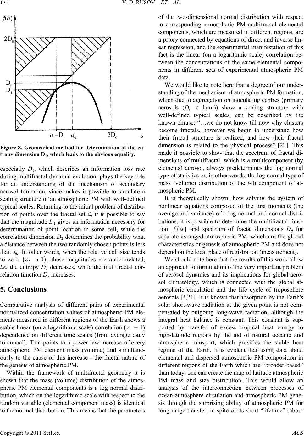




V. D. RUSOV ET AL. 132
Figure 8. Geometrical method for determination of the en-
tropy dimension D1, which leads to the obvious equality.
especially D1, which describes an information loss rate
during multifractal dynamic evolution, plays the key role
for an understanding of the mechanism of secondary
aerosol formation, since makes it possible to simulate a
scaling structure of an atmospheric PM with well-defined
ay
that the magnitude D gives an information necessary for
asured i
cales (from average daily
ints to a power law increase of every
ment mass (volume) and simultane-
usly to the cause of this increase - the fractal nature of
-multifractal elemental
co
fractal structure is realized, and how their fractal
di
typical scales. Returning to the initial problem of distribu-
tion of points over the fractal set £, it is possible to s
1
determination of point location in some cell, while the
correlation dimension D2 determines the probability what
a distance between the two randomly chosen points is less
than

L. In other words, when the relative cell size tends
to zero

0
L
 , these magnitudes are anticorrelated,
i.e. the entropy D1 decreases, while the multifractal cor-
relation function D2 increases.
5. Conclusions
Comparative analysis of different pairs of experimental
normalized concentration values of atmospheric PM ele-
ments men different regions of the Earth shows a
stable linear (on a logarithmic scale) correlation (r = 1)
dependence on different time s
to annual). That po
atmospheric PM ele
o
the genesis of atmospheric PM.
Within the framework of multifractal geometry it is
shown that the mass (volume) distribution of the atmos-
pheric PM elemental components is a log normal distri-
bution, which on the logarithmic scale with respect to the
random variable (elemental component mass) is identical
to the normal distribution. This means that the parameters
of the two-dimensional normal distribution with respect
to corresponding atmospheric PM
mponents, which are measured in different regions, are
a priory connected by equations of direct and inverse lin-
ear regression, and the experimental manifestation of this
fact is the linear (on a logarithmic scale) correlation be-
tween the concentrations of the same elemental compo-
nents in different sets of experimental atmospheric PM
data.
We would like to note here that a degree of our under-
standing of the mechanism of atmospheric PM formation,
which due to aggregation on inoculating centres (primary
aerosols (Dp  1m)) show a scaling structure with
well-defined typical scales, can be described by the
known phrase: “…we do not know till now why clusters
become fractals, however we begin to understand how
their
mension is related to the physical process” [23]. This
made it possible to show that the spectrum of fractal di-
mensions of multifractal, which is a multicomponent (by
elements) aerosol, always predetermines the log normal
type of statistics or, in other words, the log normal type of
mass (volume) distribution of the i-th component of at-
mospheric PM.
It is theoretically shown, how solving the system of
nonlinear equations composed of the first moments (the
average and variance) of a log normal and normal distri-
butions, it is possible to determine the multifractal func-
tion


f

and spectrum of fractal dimensions Dq for
separate averaged atmospheric PM, which are the global
characteristics of genesis of atmospheric PM and does not
depend on the local place of registration (measurement).
in
We should note here that the results of this work allow
an approach to formulation of the very important problem
of aerosol dynamics and its implications for global aero-
sol climatology, which is connected with the global at-
mospheric circulation and the life cycle of troposphere
aerosols [3,21]. It is known that absorption by the Earth's
solar short-wave radiation at the given point is not com-
pensated by outgoing long-wave radiation, although the
tegral heat balance is constant. This constant is sup-
ported by transfer of excess tropical heat energy to
high-latitude regions by the aid of natural oceanic and
atmospheric transport, which provides the stable heat
regime of the Earth. It is evident that using data about
elemental and dispersed atmospheric PM composition in
different regions of the Earth which are “broader-based”
than today, one can create the map of latitude atmospheric
PM mass and size distribution. This would allow an
analysis of the interconnection between processes of
ocean-atmosphere circulation and atmospheric PM gene-
sis through the surprising ability of atmospheric PM for
long range transfer, in spite of its short “lifetime” (about

V. D. RUSOV ET AL. 133
s for the plan
an
10 days) in the troposphere. If also to take into considera-
tion the evident possibility of determination of latitude
inoculating centers (i.e., primary aerosol) distribution, this
can lead to a deeper understanding of the details of aero-
sol formation and evolution, since the natural heat and
dynamic oscillations of the global ocean and atmosphere
are quite significant and should impact influence primary
aerosol formation dynamics and fractal genesis of secon-
dary atmospheric aerosol, respectively.
It is important to note also that continuous monitoring
of the main characteristics of South Pole aerosols as a
standard of relatively pure air, and the aerosols of large
cities, which are powerful sources of anthropogenic pol-
lution, allows determining the change of chemical and
dispersed compositions of aerosol pollution. Such data
are necessary for a scientifically-founded health evalua-
tion of environmental quality, as well aning
d development of an air pollution decrease strategy in
cities.
6. References
[1] W. Maenhaut and W. H. Zoller, “Determination of the
Chemical Composition of the South Pole Aerosol by in-
strumental Neutron Activation Analysis,” Journal of Ra-
dioanalytical and Nuclear Chemistry, Vol. 37, No. 2,
1977, pp. 637-650. doi:10.1007/BF02519377
[2] S. G. Pushkin and V. A. Mihaylov, “Comparative Neu-
n Analysis: Study of Atmospheric Aero-
iberian Department, Novosibirsk, 1989.
tron Activatio
sols,” Nauka, S
[3] F. Raes, R. van Dingenen, E. Vignati, J. Wilson, J. P.
Putaud, J. H. Seinfeld and P. Adams, “Formation and
Cycling of Aerosols in the Global Troposphere,” Atmos-
pheric Environment, Vol. 34, No. 25, 2000, pp. 4215-4240.
doi:10.1016/S1352-2310(00)00239-9
[4] V. D. Rusov, A. V. Glushkov and V. N. Vaschenko, “As-
trophysical Model of the Earth Global Climate,” in Rus-
sian, Naukova Dumka, Kiev, 2003.
V. Figen, Y. Narita and S. Tanaka, “The Concentratio[5] n,
Trend and Seasonal Variation of Metals in the Atmos-
phere in 16 Japanese Cities Shown by the Results of Na-
tional Air Surveillance Network (NASN) from 1974 to
1996,” Atmospheric Environment, Vol. 34, No. 17, 2000,
pp. 2755-2770.
[6] K. A. Brownlee, “Statistical Theory and Methodology in
Science and Engineering,” John Wiley & Sons, New
York, 1965.
[7] J. S. Bendat, A. G. Piersol, “Random Data: Analysis and
Measurement Procedures,” John Wiley & Sons, New
York, 1986.
[8] M. Schroeder, “Fractals, Chaos, Power Laws: Minutes
from Infinite Paradise,” W. H. Freeman and Company:
New York, 2000.
[9] T. A. Witten and L. M. Sander, “Diffusion-Limited Ag-
gregation: Kinetic Critical Phenomenon,” Physical Re-
view. Letters, Vol. 47, No. 19, 1981, pp. 1400-1403.
doi:10.1103/PhysRevLett.47.1400
[10] A. Y. Zubarev and A. O. Ivanov, “Fractal Structure of
Colloid Aggregate,” Physics and Astronomy, Vol. 47, No.
4, 2002, pp. 261-266. doi:10.1134/1.1477876
[11] W. Maenhaut, F. Francos and J. Cafmeyer, “The ‘Gent’
Stacked Filter Unit (SFU) Sampler for Collection of
mospheric Aerosols in Two Size F
At-
ractions: Description
i, S. Lands-
and Instructions for Installation and Use,” Report No.
NAHRES-19, IAEA: Vienna, 1993, pp. 249-263.
[12] P. K. Hopke, Y. Hie, T. Raunemaa, S. Biegalsk
berger, W. Maenhaut, P. Artaxo and D. Cohen, “Charac-
terization of the Gent Stacked Filter Unit PM10 Sampler,”
Aerosol Science and Technology, Vol. 27, No. 6, 1997,
pp. 726-735. doi:10.1080/02786829708965507
[13] R. Jaćimović, A. Lazaru, D. Mihajlović, R. Ilić, T. Sta-
filov, “Determination of Major and Trace Elements in
Some Minerals by k0 Instrumental Neutron Activation
Analysis,” Journal of Radioanalytical and Nuclear Che-
mistry, Vol. 253, No. 3, 2002, pp. 427-434.
doi:10.1023/A:1020421503836
[14] “HYPERMET-PC V5.0, User’s Manual,” Institute of
Isotopes, Budapest, 1997.
[15] “Kayzero/ Solcoi Version 5a. User’s Manual for Reac-
tor-neutron Activation Analysis (NAA) Using the
K0Standardization Method,” DSM Resea
2003.
rch, Geleen,
rs, Sudbury, 1995.
r, “Fractals,” Plenum Press: New York, 1988.
ntre, Mos-
rticle Size Distribution for Brownian
l of
[16] R. M. Cronover, “Introduction to Fractals and Chaos,”
Jones and Bartlett Publishe
[17] B. B. Mandelbrot, “The Fractal Geometry of Nature.
Updated and Augmented,” W. H. Freeman and Company,
New York, 2002.
[18] J. Fede
[19] S. V. Bozhokin and D. A. Parshin, “Fractals and Multi-
fractals,” in Russian, Scientific Publishing Ce
cow, 2001.
[20] F. S. Lai, S. K. Friedlander, J. Pich and G. M. Hidy, “The
Self-Preserving Pa
Coagulation in the Free-Molecular Regime,” Journa
Colloid and Interface Science, Vol. 39, No. 2, 1972, pp.
395-405. doi:10.1016/0021-9797(72)90034-3
[21] F. Raes, J. Wilsona and R. van Dingenen, “Aerosol Dy-
ory and Its
9.
namics and Its Implication for the Global Aerosol Clima-
tology,” In: R. J. Charson, J. Heintzenberg, Eds., Aerosol
Forcing of Climate, John Wiley & Sons, New York,
1995.
[22] W. Feller, “An Introduction to Probability The
Applications,” John Wiley  Sons, New York, 1971.
[23] R. Bote, R. Julen and M. Kolb, “Aggregation of Clus-
ters,” In: L. Pietronero, E. Tosatti, Eds., Fractals in Phys-
ics, North-Holland Publishing, Amsterdam, 1986, pp.
353-35
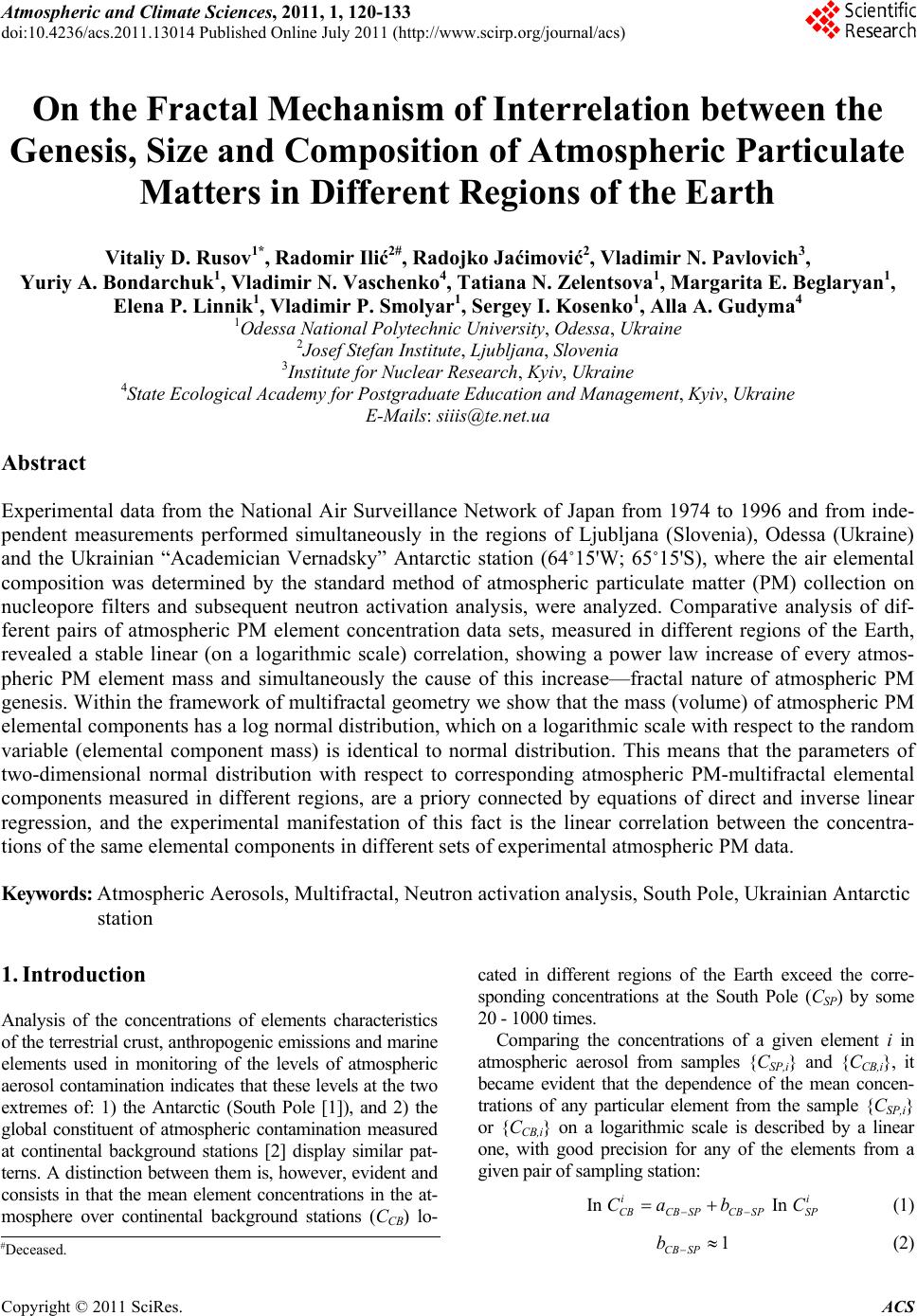