Atmospheric and Climate Sciences, 2011, 1, 134-141
doi:10.4236/acs.2011.13015 Published Online July 2011 (http://www.scirp.org/journal/acs)
Preliminary Meteorological Results of a Four-Dimensional
Data Assimilation Technique in Southern Italy
Elenio Avolio1*, S. Federico1, A. M. Sempreviva1, C. R. Calidonna1, L. De Leo1, C. Bellecci2,3
1ISAC-CNR, Lamezia Terme, Italy
2CRATI Scrl, c/o University of Calabria, Rende, Italy
3University of Rome “Tor Vergata”, Depa rt ment STFE, Rome, Italy
Received April 27, 2011; revised June 3, 2011; accepted J une 18, 2011
Abstract
A four-dimensional data assimilation (FDDA) scheme based on a Newtonian relaxation (or “nudging”) was
tested using observational asynoptic data collected at a coastal site in the Central Mediterranean peninsula of
Calabria, southern Italy. The study is referred to an experimental campaign carried out in summer 2008. For
this period a wind profiler, a sodar and two surface meteorological stations were considered. The collected
measurements were used for the FDDA scheme, and the technique was incorporated into a tailored version
of the Regional Atmospheric Modeling System (RAMS). All instruments are installed and operated routinely
at the experimental field of the CRATI-ISAC/CNR located at 600 m from the Tyrrhenian coastline. Several
simulations were performed, and the results show that the assimilation of wind and/or temperature data, both
throughout the simulation time (continuous FDDA) and for a 12 h time window (forecasting configuration),
produces improvements of the model performance. Considering a whole single day, improvements are sub-
stantial in the case of continuous FDDA while they are smaller in the case of forecasting configuration. En-
hancements, during the first six hours of each run, are generally higher. The resulting meteorological fields
are finalised as input into air quality and agro-meteorological models, for short-term predictions of renew-
able energy production forecast, and for atmospheric model initialization.
Keywords: Data Assimilation, Short Term Forecast, Mesoscale Model Performance
1. Introduction
A particularly crucial issue for improving mesoscale nu-
merical models is the improvement of knowledge of the
atmospheric state through the use of available data, in
order to produce good initial and boundary conditions.
Several instruments, such as profilers, sodars, radars,
satellite systems and surface meteorological stations, are
able to provide continuous streams of data on evolving
atmospheric conditions, and also provide spatial informa-
tion in vertical or horizontal space.
Data assimilation is the procedure that consists to in-
corporate observational data into analysis or forecast
provided by meteorological model [1].
Four Dimensional Data Assimilation (FDDA), based
on Newtonian Relaxation (or nudging) [2,3], is a useful
and relatively simple data assimilation technique to pro-
duce accurate meteorological simulations. Nudging adds
an extra tendency term to the prognostic equation of the
assimilated variable, and forces the predicted variable
towards the available observations. Since nudging is
performed toward observations, the technique is referred
to as “observational data assimilation (ODA)”
Several studies, referred to the regional and local
scales, have shown that FDDA, on average, can reduce
errors by about 25 - 60%, depending on the cases [4-7].
In this sense, the most common problem is to obtain an
independent data set for effective validation of diagnostic
models [8].
Recent studies describe experiments were verification
data differ from those used for assimilation. In Tanrikulu
et al. [9] and in Michelson and Seaman [10] is used the
data withholding technique. Also Nielsen-Gammon et al.
[11], more recently, use this approach of validation. Um-
eda and Martien [12] use different data set for verifica-
tion, and Barna and Lamb [13] perform an indirect veri-
fication, analyzing the final results of air quality simula-
tions.

E. AVOLIO ET AL. 135
In this work, we present results from a preliminary di-
rect verification approach carried out assimilating at-
mospheric parameters, both at the surface and above, at a
specific site (“LAM” experimental site). In particular, we
assimilated vertical wind profiles from the sodar and
wind profiler, and wind, temperature and specific humid-
ity from the surface meteorological station. A tailored
version of model RAMS was run at high spatial horizon-
tal resolution (1 km), to investigate the improvements of
the model performance obtained by the assimilation. The
model verification consists in comparing the simulated
parameters (in particular the surface temperature) both
with those measured in LAM station (direct and de-
pendent verification) and with those measured at a sec-
ond experimental site (“SUF” station), locate few kilo-
metres to the NE of the LAM (direct and independent
verification). The RAMS meteorological fields, simu-
lated with and without data assimilation, were evaluated
and compared for selected case studies in a 10 days stu-
dy-period, from 8 to 17 August 2008. Several experi-
ments were performed for each case (assimilation for the
entire simulation time, and for different time windows).
2. Experimental Setup
2.1. Study Area
Our analyses were conducted in the Calabria region, the
southernmost tip of the Italian peninsula located in the
Central Mediterranean Basin (Figure 1(a)). The region
extension (Figure 1(b)) ranges between 38˚12' and 40˚
latitude North and between 16˚30' and 17˚15' longitude
East. The west coast of Calabria is bounded by the Tyr-
rhenian Sea, while the East and South coasts by the
Ionian Sea. The Apennines Mountains chain runs north
to south along the coast, and the region is characterized
by five main topographical features reaching 1500 - 2000
m elevations: Pollino, Catena Costiera, Sila, Serre,
Aspromonte. The average width of the region is about 50
km in the west-east direction and 300 km in north-south
direction. There are three main planes by the sea (Sibari,
Gioa Tauro, Lamezia) where most of agricultural and
industrial areas are placed. The experimental field used
for our analysis is located in the Lamezia Plane.
2.2. Surface Stations
We considered observations from two surface stations;
the first one is located in the experimental site and is
considered both for the verification and for the assimila-
tion (“LAM” station). The second station is located few
kilometres to the NE of the experimental field and pro-
vides independent data for verification (“SUF” station).
The LAM surface station measures temperature, pres-
Figure 1. (a) Calabria region in the central Mediterranean;
(b) Calabria features cited into the text. Grey shading
shows the topographic height (m).
sure, global solar radiation, wind speed and direction (10
m above ground level), precipitation, relative humidity,
and soil temperature at 10 cm depth. The SUF station
measures only temperature, precipitation, and relative
humidity. The parameters considered for the assimila-
tions are: temperature T, relative humidity RH, and wind
W. Relative humidity, before being assimilated into the
model is converted to specific humidity. For the verifica-
tion we consider temperature only, both for LAM and
SUF station. Data are available and assimilated every 15
minutes.
2.3. Radar Wind Profiler
A radar wind profiler operated at the experimental site in
summer 2008 [14,15]. The instrument sounds the lower
troposphere, usually up to 3 km, and measures the hori-
zontal and vertical wind components using one vertical
and two oblique beams slanted at an off-zenith angle of
15.5˚. The operating frequency is 1290 MHz (about 23 cm
wavelength). Returned echoes are due to air masses re-
fractive index fluctuations generated by the wind. Data
consist of the three wind components (zonal, meridional
and vertical). The vertical resolution is 100 m, the mini-
mum range gate is 150 m, and the vertical range is 2 to 5
km depending on atmospheric conditions. Accuracy of
the wind measurements is less than 1 m/s for the hori-
zontal wind components, 0.5 m/s for the vertical compo-
nent, and less than 10˚ for the direction. Data are avail-
able every 30 minutes.
2.4. DOPPLER Sodar
Another instrument taken into account is a Doppler SO-

136 E. AVOLIO ET AL.
DAR, which operates at the experimental site [14]. The
SODAR transmits short acoustic pulses of a certain fre-
quency into the atmosphere. A small fraction of the
acoustic energy is scattered back from density fluctua-
tions in the atmosphere. Because these micro-turbulent
fluctuations move with the mean wind flow, the fre-
quency of the backscattered signal is shifted according to
the wind component parallel to the propagation of the
acoustic waves (Doppler shift). The SODAR used in this
work emits short pulses at 1900 Hz, using a phased array
with 24 loudspeakers. Measurements consist of vertical
profiles of wind speed components (horizontal and ver-
tical) and turbulence with a vertical resolution of 10 m.
The maximum vertical range is 300 m; however, the ef-
fective vertical range depends significantly on the ambi-
ent noise. The lowest range gate is 35 m. Data are avail-
able every 10 minutes.
3. Model Configuration and Simulations
3.1. RAMS Description
We used the meteorological model RAMS in its version
6.0, daily operational at ISAC-CNR (http://meteo.crati.it/
previsioni.html) and already adopted in several previous
works [16,17]. A detailed description of the RAMS
model is given in Cotton et al. [18].
The model is configured with four two-way nested
grids (Figure 2). Horizontal resolutions are 27 km, 9 km,
3 km and 1 km respectively. The fourth grid is centred
over Lamezia Terme experimental site. Thirty vertical
levels are used, from the surface up to 16,300 m of alti-
tude in the vertical coordinates that follow the terrain.
Levels are not equally spaced: layers within the Plane-
tary Boundary Layer (PBL) are between 23 and 200 m
thick, whereas layers in the middle and upper tropo-
sphere are 1000 m thick. Precipitation is calculated both
by an explicit prognostic method for seven hydrometeors
(rain, cloud droplets, hail, graupel, pristine, snow and
aggregates) and with a convective scheme that is acti-
vated for the first and the second grid. The explicit
RAMS microphysics scheme is shown in Walko et al.
[19]. Convective precipitation is parameterized following
Molinari and Corsetti [20] who proposed a simplified
form of the Kuo scheme, which includes the downdraft
effect. The parameterization of the surface layer and the
energy/momentum transfer between the atmosphere, the
biosphere and the soil, follow the LEAF-3 scheme [21].
Radiation is parameterized according to the Chen-Cotton
scheme, which includes the effect of clouds [18]. Turbu-
lent processes are calculated according to the scheme of
Mellor-Yamada [18,22], which employs a prognostic
turbulent kinetic energy.
Figure 2. RAMS model domains. Horizontal grid resolu-
tions are 27 km for the domain 1, 9 km for the domain 2, 3
km for the domain 3 and 1 km for the domain 4.
Atmospheric initial and dynamic boundary conditions
are derived from ECMWF forecast for the simulated day.
The RAMS model output is stored hourly, and each run
lasts 36 hours. We have considered 10 days, from 8 to 17
August 2008, and each day is simulated with an individ-
ual RAMS execution. Each run starting at 12 UTC of the
previous day and the first 12 h are considered for model
spin-up.
3.2. Algorithm of 4DDA (Nudging)
For the assimilation procedure, a Newtonian relaxation
(or nudging) was adopted [2,3]. The method consists of
adding a term to the prognostic equations that nudges the
predicted variables toward available observations (inter-
polated in each model grid). The nudging term is given
by:


obs m
m
t






 (1)
m

is the prognostic model variable, obs

is the
measured variable, and

is a relaxation time scale. The
relaxation time scale is chosen following empirical con-
siderations. If

is very small, the solution converges
toward the observations too fast, and the dynamics do
not have enough time to adjust; conversely, if

is too
large the errors of the model can develop too much and
the nudging does not have enough time to become effec-
tive. Several studies have demonstrated that

should
be chosen so that the last term is similar in magnitude to
the less dominant terms. Typical values of τ are between
15 minutes (strong) and 3 hours (weak). Hoke and An-

E. AVOLIO ET AL. 137
thes [23], for example, used a very short time scale (20
minutes) in their experiments, while Stauffer and Sea-
man [4] adopted about 1 hour in their work.
The spatial variation of nudging is:

0
/rr
fr e

 (2)
r is the distance from the measuring point, and 0 is
a reference distance (or radius of nudging) that repre-
sents the range of the nudging; the value = 0 corre-
sponds to the position of Lamezia Terme experimental
site. The weight of the nudging is obtained by multiply-
ing the term (1) and (2). Clearly, the choice of 0 and
r
r
r

will play a key role. After several preliminary tests
we have chosen, for our experiments, a relaxation time
scale of 900 sec. (strong nudging) and a radius of nudg-
ing of 10 km (meso-

scale).
Since the acquisition times and the spatial ranges of
the three instruments are different (Section 2). In order to
obtain a unique time of assimilation, we combined the
assimilated data as follow:
Surface station data (T, RH and W) are assimilated
every 15 minutes. At upper levels, the vertical profile of
W is obtained by combining sodar and wind profiler data
between 35 m and 200 m; above 200 m, instead, is con-
sidered only the wind profiler. First, wind profiler and
sodar measurements are averaged over 30 minutes; sub-
sequently, all the data are combined in order to build a
unique measured profile every 3 hours (00, 03, 06,..., 21
UTC), which is nudged into the model.
3.3. Simulations Description and Statistics
For each day, we have performed three numerical ex-
periments for several different cases. In particular, we
considered one simulation without assimilation (T00_
W00, corresponding to reference simulation), one simu-
lation assimilating data for the entire simulation time
(T36_W36, corresponding to continuous FDDA), and
one simulation assimilating data for a specific time win-
dow (T12_W12, corresponding to forecasting configura-
tion). It is useful to remember that each run lasts 36
hours, and the first 12 h are considered for model spin-
up.
MAE (Mean Absolute Error) and RMSE (Root Mean
Square Error) are used for statistics.
1
N
ioi
i
x
x
MAE N




(3)

2
1
N
ioi
i
xx
RMSE N




(4)
i
x
are the simulated data, oi
x
are the observations,
and is the number of data. N
MAE and RMSE are computed for T (surface temper-
ature) and for both surface stations (LAM and SUF). We
calculated the daily MAE and RMSE to estimate the
complete simulation performances, and the 6h-window
MAE and RMSE to estimate the short-term forecast per-
formances. In particular, for each day we computed the
error statistics between 00 UTC and 06 UTC for the
short-term, and between 00 UTC and 23 UTC for the
complete forecast. Obviously, T00_W00 is the reference
simulation type and all experiments are referred to it.
4. Results
Table 1 summarizes all the obtained results. To help re-
ading, we remark that:
- The upper half of the table refers to temperature
MAE, while the lower half refers to temperature RMSE;
- MAE and RMSE are reported both for LAM and for
SUF;
- For each station the error is shown for the complete
run and for the first 6 hours;
- Both for complete simulation and for the short term
forecast performances are reported errors related to T00
_W00, T36_W36 and T12_W12 experiments;
- Ten days are considered, from 8 to 17 August 2008.
Table 1 shows the error for each day, as well as their
average;
- For brevity, we focus our attention on the RMSE
only; similar conclusions can be reached by considering
the MAE. In order to catch a better confidence with the
obtained results, we calculated and show the percentage
of improvement for each run type (the calculation is per-
formed respect to the T00_W00 simulation);
- Most significant results are highlighted with letters (a,
b, c, d, e, f) and reported in bold, in the Table 1.
These results, divided for LAM and SUF station, are
summarized below.
4.1. LAM Station
Continuous FDDA (T36_W36) shows a mean RMSE re-
duction of 41% (a) for the complete run, and 63% (b) for
the first 6 hours of simulation. The result (a) can be con-
sidered as representative of the improvement in the pro-
duction of mesoscale analysis.
Forecasting configuration FDDA (T12_W12) shows a
mean RMSE reduction of 16% (c) for the whole run, and
35% (d) for the first 6 hours. The result (d) can be con-
sidered as representative of the improvement in short-
erm prediction. t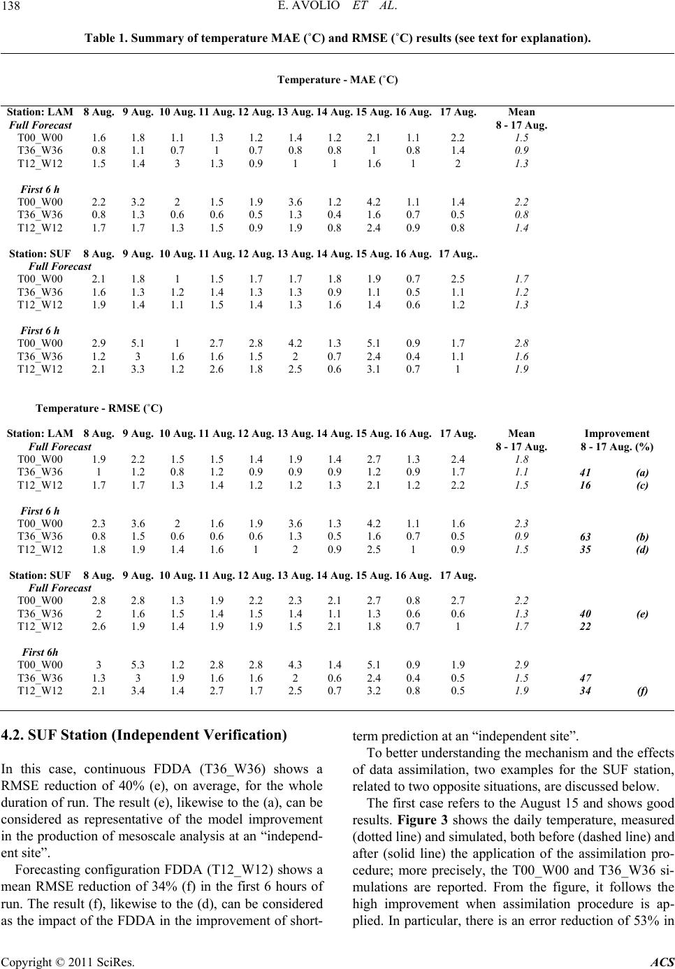

E. AVOLIO ET AL. 138
Table 1. Summary of temperature MAE (˚C) and RMSE (˚C) results (see text for explanation).
Temp eratur e - MAE (˚C)
Station: LAM 8 Aug. 9 Aug. 10 Aug. 11 Aug. 12 Aug.13 Aug.14 Aug.15 Aug.16 Aug.17 Aug.
Full Forecast Mean
8 - 17 Aug.
T00_W00 1.6 1.8 1.1 1.3 1.2 1.4 1.2 2.1 1.1 2.2 1.5
T36_W36 0.8 1.1 0.7 1 0.7 0.8 0.8 1 0.8 1.4 0.9
T12_W12 1.5 1.4 3 1.3 0.9 1 1 1.6 1 2 1.3
First 6 h
T00_W00 2.2 3.2 2 1.5 1.9 3.6 1.2 4.2 1.1 1.4 2.2
T36_W36 0.8 1.3 0.6 0.6 0.5 1.3 0.4 1.6 0.7 0.5 0.8
T12_W12 1.7 1.7 1.3 1.5 0.9 1.9 0.8 2.4 0.9 0.8 1.4
Station: SUF 8 Aug. 9 Aug. 10 Aug. 11 Aug. 12 Aug.13 Au g .14 Aug.15 Aug.16 Aug.17 A ug..
Full Forecast
T00_W00 2.1 1.8 1 1.5 1.7 1.7 1.8 1.9 0.7 2.5 1.7
T36_W36 1.6 1.3 1.2 1.4 1.3 1.3 0.9 1.1 0.5 1.1 1.2
T12_W12 1.9 1.4 1.1 1.5 1.4 1.3 1.6 1.4 0.6 1.2 1.3
First 6 h
T00_W00 2.9 5.1 1 2.7 2.8 4.2 1.3 5.1 0.9 1.7 2.8
T36_W36 1.2 3 1.6 1.6 1.5 2 0.7 2.4 0.4 1.1 1.6
T12_W12 2.1 3.3 1.2 2.6 1.8 2.5 0.6 3.1 0.7 1 1.9
Temperature - RMSE (˚C)
Station: LAM 8 Aug. 9 Aug. 10 Aug. 11 Aug. 12 Aug.13 Aug.14 Aug.15 Aug.16 Aug.17 Aug.
Full Forecast Mean 8 - 17 Aug. Improvement 8 - 17 Aug. (%)
T00_W00 1.9 2.2 1.5 1.5 1.4 1.9 1.4 2.7 1.3 2.4 1.8
T36_W36 1 1.2 0.8 1.2 0.9 0.9 0.9 1.2 0.9 1.7 1.1 41 (a)
T12_W12 1.7 1.7 1.3 1.4 1.2 1.2 1.3 2.1 1.2 2.2 1.5 16 (c)
First 6 h
T00_W00 2.3 3.6 2 1.6 1.9 3.6 1.3 4.2 1.1 1.6 2.3
T36_W36 0.8 1.5 0.6 0.6 0.6 1.3 0.5 1.6 0.7 0.5 0.9 63 (b)
T12_W12 1.8 1.9 1.4 1.6 1 2 0.9 2.5 1 0.9 1.5 35 (d)
Station: SUF 8 Aug. 9 Aug. 10 Aug. 11 Aug. 12 Aug.13 Aug.14 Aug.15 Aug.16 Aug.17 Aug.
Full Forecast
T00_W00 2.8 2.8 1.3 1.9 2.2 2.3 2.1 2.7 0.8 2.7 2.2
T36_W36 2 1.6 1.5 1.4 1.5 1.4 1.1 1.3 0.6 0.6 1.3 40 (e)
T12_W12 2.6 1.9 1.4 1.9 1.9 1.5 2.1 1.8 0.7 1 1.7 22
First 6h
T00_W00 3 5.3 1.2 2.8 2.8 4.3 1.4 5.1 0.9 1.9 2.9
T36_W36 1.3 3 1.9 1.6 1.6 2 0.6 2.4 0.4 0.5 1.5 47
T12_W12 2.1 3.4 1.4 2.7 1.7 2.5 0.7 3.2 0.8 0.5 1.9 34 (f)
4.2. SUF Station (Independent Verification)
In this case, continuous FDDA (T36_W36) shows a
RMSE reduction of 40% (e), on average, for the whole
duration of run. The result (e), likewise to the (a), can be
considered as representative of the model improvement
in the production of mesoscale analysis at an “independ-
ent site”.
Forecasting configuration FDDA (T12_W12) shows a
mean RMSE reduction of 34% (f) in the first 6 hours of
run. The result (f), likewise to the (d), can be considered
as the impact of the FDDA in the improvement of short-
term prediction at an “independent site”.
To better understanding the mechanism and the effects
of data assimilation, two examples for the SUF station,
related to two opposite situations, are discussed below.
The first case refers to the August 15 and shows good
results. Figure 3 shows the daily temperature, measured
(dotted line) and simulated, both before (dashed line) and
after (solid line) the application of the assimilation pro-
cedure; more precisely, the T00_W00 and T36_W36 si-
mulations are reported. From the figure, it follows the
high improvement when assimilation procedure is ap-
plied. In particular, there is an error reduction of 53% in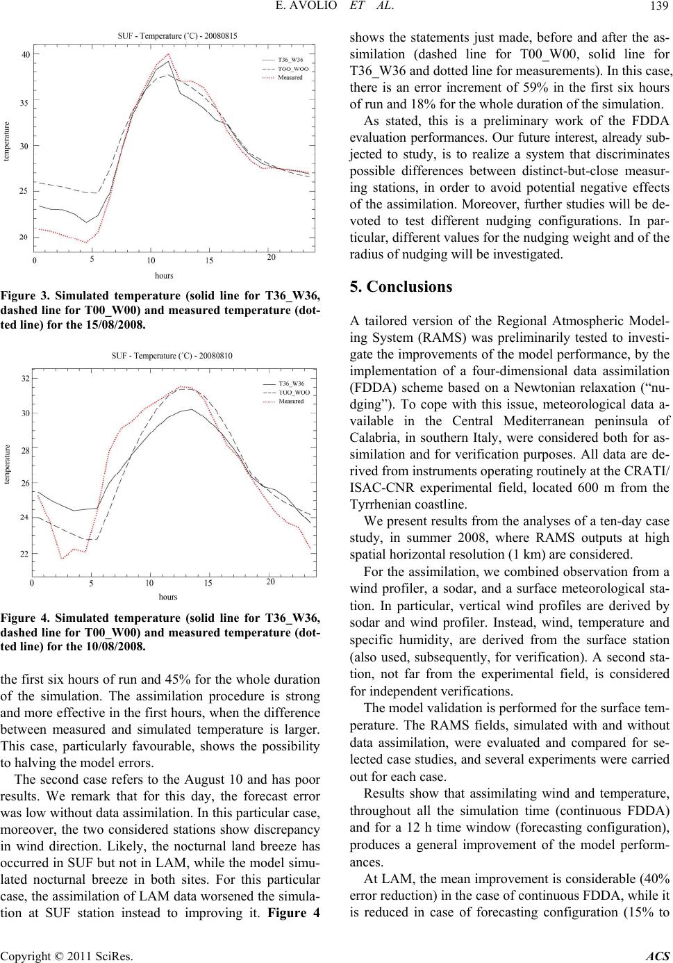

E. AVOLIO ET AL. 139
Figure 3. Simulated temperature (solid line for T36_W36,
dashed line for T00_W00) and measured temperature (dot-
ted line) for the 15/08/2008.
Figure 4. Simulated temperature (solid line for T36_W36,
dashed line for T00_W00) and measured temperature (dot-
ted line) for the 10/08/2008.
the first six hours of run and 45% for the whole duration
of the simulation. The assimilation procedure is strong
and more effective in the first hours, when the difference
between measured and simulated temperature is larger.
This case, particularly favourable, shows the possibility
to halving the model errors.
The second case refers to the August 10 and has poor
results. We remark that for this day, the forecast error
was low without data assimilation. In this particular case,
moreover, the two considered stations show discrepancy
in wind direction. Likely, the nocturnal land breeze has
occurred in SUF but not in LAM, while the model simu-
lated nocturnal breeze in both sites. For this particular
case, the assimilation of LAM data worsened the simula-
tion at SUF station instead to improving it. Figure 4
shows the statements just made, before and after the as-
similation (dashed line for T00_W00, solid line for
T36_W36 and dotted line for measurements). In this case,
there is an error increment of 59% in the first six hours
of run and 18% for the whole duration of the simulation.
As stated, this is a preliminary work of the FDDA
evaluation performances. Our future interest, already sub-
jected to study, is to realize a system that discriminates
possible differences between distinct-but-close measur-
ing stations, in order to avoid potential negative effects
of the assimilation. Moreover, further studies will be de-
voted to test different nudging configurations. In par-
ticular, different values for the nudging weight and of the
radius of nudging will be investigated.
5. Conclusions
A tailored version of the Regional Atmospheric Model-
ing System (RAMS) was preliminarily tested to investi-
gate the improvements of the model performance, by the
implementation of a four-dimensional data assimilation
(FDDA) scheme based on a Newtonian relaxation (“nu-
dging”). To cope with this issue, meteorological data a-
vailable in the Central Mediterranean peninsula of
Calabria, in southern Italy, were considered both for as-
similation and for verification purposes. All data are de-
rived from instruments operating routinely at the CRATI/
ISAC-CNR experimental field, located 600 m from the
Tyrrhenian coastline.
We present results from the analyses of a ten-day case
study, in summer 2008, where RAMS outputs at high
spatial horizontal resolution (1 km) are considered.
For the assimilation, we combined observation from a
wind profiler, a sodar, and a surface meteorological sta-
tion. In particular, vertical wind profiles are derived by
sodar and wind profiler. Instead, wind, temperature and
specific humidity, are derived from the surface station
(also used, subsequently, for verification). A second sta-
tion, not far from the experimental field, is considered
for independent verifications.
The model validation is performed for the surface tem-
perature. The RAMS fields, simulated with and without
data assimilation, were evaluated and compared for se-
lected case studies, and several experiments were carried
out for each case.
Results show that assimilating wind and temperature,
throughout all the simulation time (continuous FDDA)
and for a 12 h time window (forecasting configuration),
produces a general improvement of the model perform-
ances.
At LAM, the mean improvement is considerable (40%
error reduction) in the case of continuous FDDA, while it
is reduced in case of forecasting configuration (15% to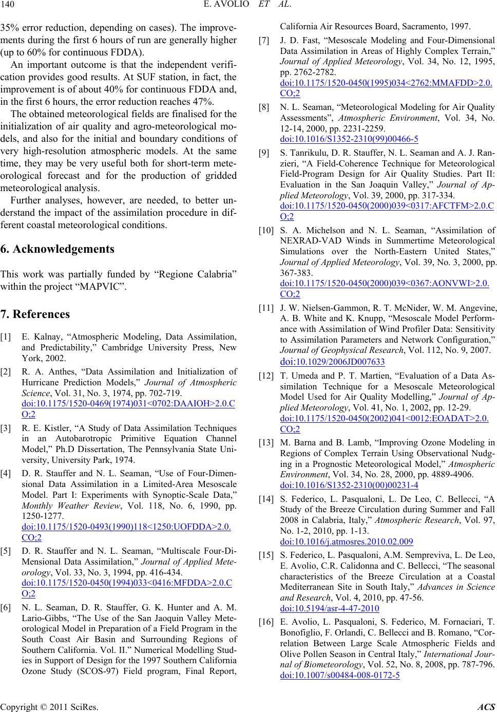

140 E. AVOLIO ET AL.
35% error reduction, depending on cases). The improve-
ments during the first 6 hours of run are generally higher
(up to 60% for continuous FDDA).
An important outcome is that the independent verifi-
cation provides good results. At SUF station, in fact, the
improvement is of about 40% for continuous FDDA and,
in the first 6 hours, the error reduction reaches 47%.
The obtained meteorological fields are finalised for the
initialization of air quality and agro-meteorological mo-
dels, and also for the initial and boundary conditions of
very high-resolution atmospheric models. At the same
time, they may be very useful both for short-term mete-
orological forecast and for the production of gridded
meteorological analysis.
Further analyses, however, are needed, to better un-
derstand the impact of the assimilation procedure in dif-
ferent coastal meteorological conditions.
6. Acknowledgements
This work was partially funded by “Regione Calabria”
within the project “MAPVIC”.
7. References
[1] E. Kalnay, “Atmospheric Modeling, Data Assimilation,
and Predictability,” Cambridge University Press, New
York, 2002.
[2] R. A. Anthes, “Data Assimilation and Initialization of
Hurricane Prediction Models,” Journal of Atmospheric
Science, Vol. 31, No. 3, 1974, pp. 702-719.
doi:10.1175/1520-0469(1974)031<0702:DAAIOH>2.0.C
O;2
[3] R. E. Kistler, “A Study of Data Assimilation Techniques
in an Autobarotropic Primitive Equation Channel
Model,” Ph.D Dissertation, The Pennsylvania State Uni-
versity, University Park, 1974.
[4] D. R. Stauffer and N. L. Seaman, “Use of Four-Dimen-
sional Data Assimilation in a Limited-Area Mesoscale
Model. Part I: Experiments with Synoptic-Scale Data,”
Monthly Weather Review, Vol. 118, No. 6, 1990, pp.
1250-1277.
doi:10.1175/1520-0493(1990)118<1250:UOFDDA>2.0.
CO;2
[5] D. R. Stauffer and N. L. Seaman, “Multiscale Four-Di-
Mensional Data Assimilation,” Journal of Applied Mete-
orology, Vol. 33, No. 3, 1994, pp. 416-434.
doi:10.1175/1520-0450(1994)033<0416:MFDDA>2.0.C
O;2
[6] N. L. Seaman, D. R. Stauffer, G. K. Hunter and A. M.
Lario-Gibbs, “The Use of the San Jaoquin Valley Mete-
orological Model in Preparation of a Field Program in the
South Coast Air Basin and Surrounding Regions of
Southern California. Vol. II.” Numerical Modelling Stud-
ies in Support of Design for the 1997 Southern California
Ozone Study (SCOS-97) Field program, Final Report,
California Air Resources Board, Sacramento, 1997.
[7] J. D. Fast, “Mesoscale Modeling and Four-Dimensional
Data Assimilation in Areas of Highly Complex Terrain,”
Journal of Applied Meteorology, Vol. 34, No. 12, 1995,
pp. 2762-2782.
doi:10.1175/1520-0450(1995)034<2762:MMAFDD>2.0.
CO;2
[8] N. L. Seaman, “Meteorological Modeling for Air Quality
Assessments”, Atmospheric Environment, Vol. 34, No.
12-14, 2000, pp. 2231-2259.
doi:10.1016/S1352-2310(99)00466-5
[9] S. Tanrikulu, D. R. Stauffer, N. L. Seaman and A. J. Ran-
zieri, “A Field-Coherence Technique for Meteorological
Field-Program Design for Air Quality Studies. Part II:
Evaluation in the San Joaquin Valley,” Journal of Ap-
plied Meteorology, Vol. 39, 2000, pp. 317-334.
doi:10.1175/1520-0450(2000)039<0317:AFCTFM>2.0.C
O;2
[10] S. A. Michelson and N. L. Seaman, “Assimilation of
NEXRAD-VAD Winds in Summertime Meteorological
Simulations over the North-Eastern United States,”
Journal of Applied Meteorology, Vol. 39, No. 3, 2000, pp.
367-383.
doi:10.1175/1520-0450(2000)039<0367:AONVWI>2.0.
CO;2
[11] J. W. Nielsen-Gammon, R. T. McNider, W. M. Angevine,
A. B. White and K. Knupp, “Mesoscale Model Perform-
ance with Assimilation of Wind Profiler Data: Sensitivity
to Assimilation Parameters and Network Configuration,”
Journal of Geophysical Research, Vol. 112, No. 9, 2007.
doi:10.1029/2006JD007633
[12] T. Umeda and P. T. Martien, “Evaluation of a Data As-
similation Technique for a Mesoscale Meteorological
Model Used for Air Quality Modelling,” Journal of Ap-
plied Meteorology, Vol. 41, No. 1, 2002, pp. 12-29.
doi:10.1175/1520-0450(2002)041<0012:EOADAT>2.0.
CO;2
[13] M. Barna and B. Lamb, “Improving Ozone Modeling in
Regions of Complex Terrain Using Observational Nudg-
ing in a Prognostic Meteorological Model,” Atmospheric
Environment, Vol. 34, No. 28, 2000, pp. 4889-4906.
doi:10.1016/S1352-2310(00)00231-4
[14] S. Federico, L. Pasqualoni, L. De Leo, C. Bellecci, “A
Study of the Breeze Circulation during Summer and Fall
2008 in Calabria, Italy,” Atmospheric Research, Vol. 97,
No. 1-2, 2010, pp. 1-13.
doi:10.1016/j.atmosres.2010.02.009
[15] S. Federico, L. Pasqualoni, A.M. Sempreviva, L. De Leo,
E. Avolio, C.R. Calidonna and C. Bellecci, “The seasonal
characteristics of the Breeze Circulation at a Coastal
Mediterranean Site in South Italy,” Advances in Science
and Research, Vol. 4, 2010, pp. 47-56.
doi:10.5194/asr-4-47-2010
[16] E. Avolio, L. Pasqualoni, S. Federico, M. Fornaciari, T.
Bonofiglio, F. Orlandi, C. Bellecci and B. Romano, “Cor-
relation Between Large Scale Atmospheric Fields and
Olive Pollen Season in Central Italy,” International Jour-
nal of Biometeorology, Vol. 52, No. 8, 2008, pp. 787-796.
doi:10.1007/s00484-008-0172-5

E. AVOLIO ET AL. 141
[17] S. Federico, E. Avolio, C. Bellecci and M. Colacino,
“The Meteorological Model RAMS at Crati Scrl,” Ad-
vances in Geosciences, Vol. 2, 2005, pp. 177-180.
doi:10.5194/adgeo-2-177-2005
[18] W. R. Cotton, R. A. Pielke Sr., R. L. Walko, G. E. Liston,
C. J. Tremback, H. Jiang, R. L. McAnelly, J. Y. Harring-
ton, M. E. Nicholls, G. G. Carrio, J. P. McFadden,
“RAMS 2001: Current Status and Future Directions,”
Meteorology and Atmosphere Physics, Vol. 82, No. 1-4,
2003, pp. 5-29. doi:10.1007/s00703-001-0584-9
[19] R. L. Walko, W. R. Cotton, M. P. Meyers, J. Y. Harring-
ton, “New RAMS Cloud Microphysics Parameterization
Part I: The Single-Moment Scheme,” Atmosphere Re-
search, Vol. 38, No. 1-4, 2995, pp. 29-62.
doi:10.1016/0169-8095(94)00087-T
[20] J. Molinari and T. Corsetti, “Incorporation of
Cloud-Scale and Mesoscale Down-Drafts Into A Cumu-
lus Parameterization: Results of One and
Three-Dimensional Integrations,” Monthly Weather Re-
view, Vol. 113, No. 4, 1985, pp. 485-501.
doi:10.1175/1520-0493(1985)113<0485:IOCSAM>2.0.C
O;2
[21] R. L. Walko, L. E. Band, J. Baron, T. G. Kittel, R. Lam-
mers, T. J. Lee, D. Ojima, R. A. Sr. Pielke, C. Taylor, C.
Tague, C. J. Tremback and P. L. Vidale, “Coupled At-
mosphere-Biosphere-Hydrology Models for Environ-
mental Prediction,” Journal of Applied Meteorology, Vol.
39, No. 6, 2000, pp. 931-944.
doi:10.1175/1520-0450(2000)039<0931:CABHMF>2.0.
CO;2
[22] G. Mellor and T. Yamada, “Development of a Turbulence
Closure Model for Geophysical Fluid Problems,” Reviews
of Geophysics and Space Physics, Vol. 20, No. 4, 1982,
pp. 851-875. doi:10.1029/RG020i004p00851
[23] J. E. Hoke and R. A. Anthes, “Initialization of numerical
Models by a Dynamic-Initialization Technique,” Monthly
Weather Review, Vol. 104, No. 12, 1976, pp. 1551-1556.
doi:10.1175/1520-0493(1976)104<1551:TIONMB>2.0.C
O;2
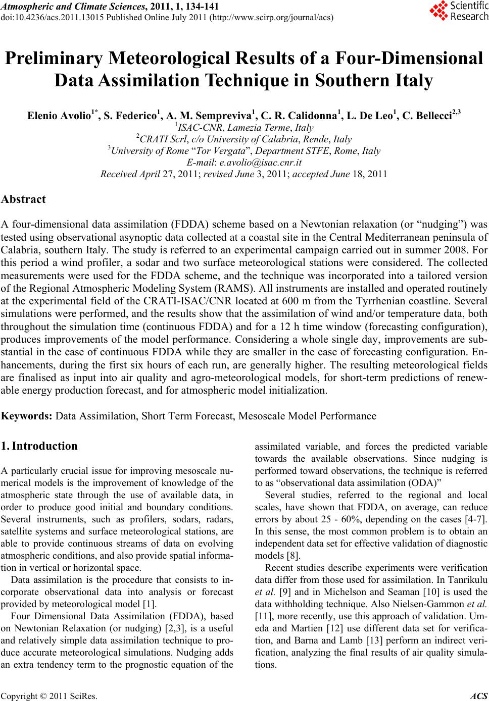