Journal of Computer and Communications, 2015, 3, 198-204
Published Online November 2015 in SciRes. http://www.scirp.org/journal/jcc
http://dx.doi.org/10.4236/jcc.2015.311031
How to cite this paper: Choudhury, A. and Nagaswamy, S. (2015) A Bayesian Approach to Identify Photos Likely to Be More
Popular in Social Media. Journal of Computer and Communications, 3, 198-204. http://dx.doi.org/10.4236/jcc.2015.311031
A Bayesian Approach to Identify Photos
Likely to Be More Popular in
Social Media
Arunabha Choudhury, Sriram Nagaswamy
Samsung R and D, Bangalore, India
Received Novemb er 20 15
Abstract
With cameras becoming ubiquitous in Smartphones, it has become a very common trend to cap-
ture and share moments with friends and family in social media. Arguably, the 2 most relevant
factors that contribute to the popularity are: the user’s social aspect and the content of the image
(image quality, objects in the image etc.). In recent years, due to various security concerns, it has
been increasingly difficult to derive social attributes from social media. Due to this limitation, in
this paper we study what make images popular in social media based on the image content alone.
We use Bayesian learning approach with variable likelihood function in order to predict image
popularity. Our finding shows that a mapping between image content to image popularity can be
achieved with a significant recall and precision. We then use our model to predict images that are
likely to be more popular from a set of user images which eventually facilitate easy share.
Keywords
Bayesian, Supervised Learning, Image Popularity, Classification, Data Mining
1. Introduction
Image popularity for a user in social media can be attributed to variety of factors of which both image content as
well as the social aspect plays significant role. With the explosion in number of photos clicked using Smart-
phones, it is important that the user can quickly search and find photos he may be interested in. According to
report from KPCB analyst Mary Meeker in 2014, we now upload and share over 1.8 billion photos each day
through various channels and social media. Since the numbers of people who have access to these images are
also very large, getting one’s image viewed or liked by many people gives a feeling of being popular in one’s
social circle and in turn an instant gratification. This makes image popularity an important driving factor for
choosing and sharing the right image from a large collection of images. In this research we investigate what im-
ages are likely to be more popular so that a recommendation channel can be generated to allow the user to
quickly access these photos.
Even though popularity of text (such as tweets) [1] [2] and videos (such as YouTube videos) [3]-[5] have
been studied in recent years, image popularity prediction still remains a difficult problem. In our study, we have

A. Choudhury, S. Nagaswamy
199
found that the most relevant research work in image popularity prediction [6] has been done using the Flickr da-
taset. This research is however a combination of both social aspects and image content. Also, the definition of
popularity is number of views in Flickr. As opposed to these ideas, in our work, we address two issues in partic-
ular: First, we investigate whether there is a more relevant definition of image popularity and answer this ques-
tion affirmatively. Second, we show that it is possible to predict image popularity with a significant accuracy
based on image content alone. Although our definition of popularity is based on number of likes in Facebook,
we have only used this information to label the training set. To the best of our knowledge, this work is the first
to predict image popularity based on image content alone.
2. Related Work
As already discussed, the most significant work on image popularity prediction has been done by Khosla et al.
[6]. For other related work on popularity, there has been some work by Figueiredo et al. in video popularity pre-
diction [7] [8]. However, their work is mostly dependent on social aspect like comments and tags associated
with videos. Popularity prediction has been studied in other areas like popularity of online articles [9] and popu-
larity of social marketing messages [10]. However, the study done in these papers comes under the category of
predicting text popularity such as tweets or Facebook posts and predicting popularity of web pages. None of
these in any way relate to the image popularity we discuss in this work. Xinran et al. in [11] have studied the
prediction of clicks on Ads in Facebook as a classification problem. Although number of clicks associated with
an ad can be considered as a form of popularity, click prediction of an Ad is not directly related to popularity.
In another interesting work by Justin Cheng et al. in [12] they study the prediction of cascading in social me-
dia such as Twitter and Facebook. Cascading refers to sharing and re-sharing posts in Facebook and re-tweeting
tweets in Twitter. These sharing may include anything from text to images that is sharable through these chan-
nels. The growth of this cascade can also in some ways be considered as popularity of the sharable items. This
however does not directly relate to our consideration of image popularity for individual users in social media
particularly for two reasons. First, most of these sharable items consist of items that are strictly public and not
private images from users. Second, along with content, there is a strict dependency on other social features that
cannot easily be avoided. Although a separate study of popularity prediction for these sharable items is possible,
in our context, due to their varied properties we have decided not to mix them up.
3. Regression vs. Classification
The definition of popularity by Khosla et al. in [6] is number of views in Flickr. In their work they have consi-
dered the normalized view count as the dependent variable for regression and the performance measure is in
terms of rank correlation. Table 1 summarizes their results.
From Table 1, one can see that the contribution to prediction by image content alone is very low and most of
the contribution is from social aspect. Another issue is the number of features used in [6] is very large for image
content alone and yet contribution to prediction from all these features is very little. Table 2 summarizes this
issue.
Table 1. Rank correlation for image content and social attributes in [6].
Dataset Type Image Content Only Social Attributes Only Content + Social
One-per-user 0.31 0.77 0.81
User-mix 0.36 0.66 0.72
User-specific 0.40 0.21 0.48
Table 2. Rank correlation for individual feature type and combined [6].
Dataset Type Gist Color Histogram Texture Color Patches Gradient Deep Learning Objects Combined
One-per-user 0.07 0.12 0.20 0.23 0.26 0.28 0.23 0.31
User-mix 0.13 0.15 0.22 0.29 0.32 0.33 0.30 0.36
User-specific 0.16 0.23 0.32 0.36 0.34 0.26 0.33 0.40

A. Choudhury, S. Nagaswamy
200
Each of these categories in image content (like Gist, Texture etc.) consists of a number of features ranging
from 512 to 10,752. Computing all these features from a collection of images may not be a feasible scenario in
devices such as Smartphones where one is limited in terms of memory and processing capabilities. Also in [6]
the final prediction is number of views an image is likely to receive as a result of prediction but the conclusion
whether or not the image is popular is a matter of subjective judgment (one may decide popularity based on
number of predicted view count). In our work we look at this problem in slightly different way.
3.1. Definition of Image Popularity
As already mentioned in [6] there are various ways to define popularity. In our work we use the number of likes
in Facebook as a measure of popularity. Since “Like” in Facebook refers to users consciously making a decision
of whether or not they “Like” an image, in our consideration this definition is slightly better than number of
views, which may be noisier in certain situation. Nonetheless, the definition of true popularity may still be ar-
gued and remains a difficult question to answer.
For our purpose, the raw like count cannot directly be used as measure of popularity. The reason being, in
Facebook only people friends with the users are allowed to like photos. Thus, people with low friend count may
have images which are popular in their circle but may not match up to the like count for users with many friends.
For this reason we have normalized the like count per user basis. Figure 1 shows the density plot for number of
likes and number of likes normalized.
As expected, we see from Figure 1 that the median normalized like count is about 0.1 and about a quarter of
images have normalized like count more than 0.4. One can at this point consider 0.4 as the threshold to define
popularity of an image. This definition of popularity however may still be improved. The third quartile threshold
based on the entire collection is still subjected to the fact that popularity of an image is across multiple users. As
already discussed, each user in Facebook may have a local sense of popularity for which the above definition
may still affect images when the variance in like count is high between users with high and low friend count. In
order to overcome this issue and to consider local popularity as the measure of popularity, we first find the mean
of normalized like count for each user. Then, for each user, if an image has normalized like count more than the
mean, we consider that image to be popular. Figure 2 gives the boxplot for normalized like count for random
users chosen from the dataset.
From Figure 2 we can see that in many cases the distribution of normalized like count for users are skewed.
Here one may argue median to be a better estimate. But in our observation we have seen that for most cases the
distribution is right skewed. Hence mean gives a tighter bound than median. This is shown in Figure 3. As we
can see in most cases mean is either comparable to median or more than median. Hence, for our purpose we
consider mean normalized like count for each user to be our threshold for popularity.
Figure 1. Density plot.
Figure 2. Boxplot for normalized like count (22 random users).

A. Choudhury, S. Nagaswamy
201
Figure 3. Mean vs median for normalized like count (22 random users).
3.2. Dataset
In this section we introduce the dataset and the features we have used for our experiment. Firstly, our data set
comprises of user images from Facebook with number of likes for each image as the measure of popularity. For
our analysis, we have collected about 1000 images from 35 different Facebook users. We normalized the like
count for each user. We then convert the like count to a binary label 0 and 1 with 0 being the like count less than
the mean normalized like count and 1 being like count more than the mean normalized like count for each user.
Secondly, our final feature set after feature selection consists of eight low level computer vision features called
blur, motion blur, brightness, overexposure, underexposure, contrast, feature number, out of focus background
and one high level image feature whose values have been derived from face size and number of faces in the im-
age. The first eight features are more relevant to the quality of the image whereas the last one correspond to ob-
jects in the image; in this case faces. Our assumption is that quality of image is a very important factor for im-
ages being popular but not the only factor. Presence of faces in the image in social media makes a big difference
and hence, we have also considered face size and number of faces in the image.
3.3. Regression
We first use the normalized like count as it is to predict the number of likes for each image. Table 3 summarizes
the performance in terms of rank correlation for SVR, Linear regression and ANN.
As we can see, the rank correlation using only nine features are comparable to the rank correlation in Table 2.
Therefore, using image content alone may not be sufficient for this regression problem. Thus, for our purpose,
we convert this problem to a classification problem by converting the normalized like count to popularity. The
conversion is according to the definition of popularity introduced in Section 3.2.
3.4. Classification
We then try to formalize this problem as a binary classification problem with,
{ }
12
,,,
d
X xxx= …
the image data and
j
x
the
th
j
feature vector
{ }
12
,B yy=
the set of binary labels
D
a given distribution over
T
XB×
The goal is to find a function f such that minimizes
(,)~
[ ()]
xy D
Efx y≠
(1)
where,
(,)~ xy D
E
is an error function [13] that calculates error between original class label y and predicted labels
()fx
. We then train six different supervised learning algorithms. Test results are given in terms of precision,
recall and accuracy and are averaged over twenty trials. These results are plotted in Figure 4. Here we can see
that the classification accuracy is more or less uniform across all classifiers. Hence, in order to differentiate their
performance we also plot precision and recall for all classifiers in Figure 4.
Since in our case it is more appropriate to weight both precision and recall equally, we consider f-measure as
our performance matrix. In Figure 5 we plot the f-measure for all the classifiers for eight random trials. From
the plots we observe that performance of Naïve Bayes is relatively more consistent. Even though ANN does
better in some cases the performance is not very consistent. For the purpose of consistency and overall perfor-
mance measure we have considered Naïve Bayes as our base model.
0
0.5
1
1
3
5
7
9
11
13
15
17
19
21
Mean
Median

A. Choudhury, S. Nagaswamy
202
Figure 4. Performance plot for different classifiers.
Figure 5. Plot of f-measure.
Table 3. Rank correlation for different regression algorithms.
Regression model Correlation
SVR 0.22
Linear regression 0.20
ANN 0.23
4. Experiment
For a given set of feature vector X and binary label set B Bayes theorem can be stated as:
() ( )
| ()
|()
XB
BX
fxBy fy
f yXxfx
=
= =
( 2)
where,
( )
|
X
fxB y=
is the conditional density function. In our Naïve Bayes implementation in the previous
section, the assumption is that
()( )
|~ ,,
X
fxB yNx µσ = ∀
(3)

A. Choudhury, S. Nagaswamy
203
In order to verify this we plot the density function of one of the features Blur in Figure 6.
For a lot of features in our case the Normal distribution turns out to be a not so good fit. In our experiment we
also observe that for certain features a Gamma or a Weibull distribution fits better than Normal distribution. Ta-
ble 4 summarizes this observation.
We measure goodness of fit in terms of p-value greater than 0.05. From the summary in Table 4 we can see
that some features even though fit well with Normal distribution, in other cases Weibull or Gamma distribution
scores higher in terms of goodness of fit (Figure 6 and Figure 7).
We finally use this variable density function based Naïve Bayes to predict popularity. Figu re 8 compares the
precision and recall of Naïve Bayes with normal distribution (NBND) vs. Naïve Bayes with variable density
function (NBVDF). With this modification we have been able to achieve a 52% precision and 80% recall.
Figure 6. Blur density plot with Normal and Weibull distribution respectively (red).
Figure 7. Contrast density plot with Gamma distribution (red).
Figure 8. Naïve Bayes (normal vs. variable distribution).

A. Choudhury, S. Nagaswamy
204
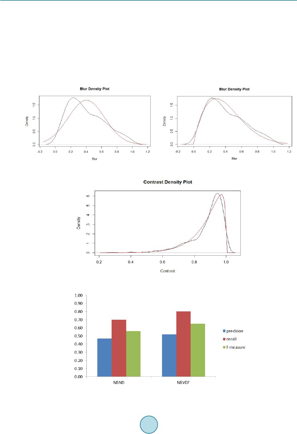
Table 4. Goodness of fit (p-values) .
Features Normal Gamma Weibull
Brightness 0.641 0.003 0.60
Blur 0.0 0.175 0.455
Motion Blur 0.004 0.036 0.703
Over Exposure 0.0 0.0 0.228
Contrast 0.0 0.047 0.034
5. Conclusion
A regression based popularity prediction has constrains such as: low accuracy when only image content is used,
system overhead due to large number of features and highly dependent on social data which may not always be
available. In most cases one is concerned with the final decision on whether or not an image is going to be pop-
ular and not be concerned about the number of views or likes. Thus solving the classification problem is much
more intuitive and a simple Naïve Bayes variant works well without much system overhead. In future we plan to
add contextual information to improve the overall precision and recall. In our work we have been able to show
that one may choose to ignore any social aspect associated with the image and still achieve significant precision
and recall to predict popularity of an image purely based on image features.
References
[1] Petrovic, S., Osborne, M. and Lavrenko, V. (2011) Rt to Win! Predicting Message Propagation in Twitter. ICWSM.
[2] Hong, L., Dan, O. and Davison, B.D. (2011) Predicting Popular Messages in Twitter. WWW (Companion Volume),
57-58. http://dx.doi.org/10.1145/1963192.1963222
[3] Pinto, H. , Almeida, J.M. and Goncalves, M.A. (2013) Using Early View Patterns to Predict the Popularity of Youtube
Videos. WSDM, 365-374.
[4] Shamma, D.A., Yew, J., Kennedy, L. and Churchill, E.F. (2011) Viral Actions: Predicting Video View Counts Using
Synchronous Sharing Behaviors. ICWSM.
[5] Nwana, A.O., Avestimehr, S. and Chen, T. (2013) A Latent Social Approach to Youtube Popularity Prediction. C oRR .
[6] Khosla, A., Sarma, A.D. and Hamid, R. (2014) What Makes an Image Popular? IW3C2.
[7] Figueiredo, F. (2013) On the Prediction of Popularity of Trends and Hits for User Generated Videos. Proceedings of
the Sixth ACM International Conference on Web Search and Data Mining, 741-746.
http://dx.doi.org/10.1145/2433396.2433489
[8] Figueiredo, F., Benevenuto, F. and Almeida, J.M. (2011) The Tube over Time: Characterizing Popularity Growth of
YouTube Videos. Proceedings of the Fourth ACM International Conference on Web Search and Data Mining, 745-
754. http://dx.doi.org/10.1145/1935826.1935925
[9] Vanwinckelen, G. and Meert, W. (2014) Predicting the Popularity of Online Articles with Random Forests. ECML/
PKDD Discovery Challenge on Predictive Web Analytics, Nancy, September 2014.
[10] Yu, B., Chen, M. and Kwok, L. (2011) Toward Predicting Popularity of Social Marketing Messages. Salerno, J., et al.,
Eds., SBP 2011, LNCS 6589, 317-324. http://dx.doi.org/10.1007/978-3-642-19656-0_44
[11] He, X., et al. (2014) Practical Lessons from Predicting Clicks on Ads at Facebook. ADKDD’14, 24-27 August 2014.
http://dx.doi.org/10.1145/2648584.2648589
[12] Cheng, J., Adamic, L.A. , Dow, P.A., Kleinberg, J. and Leskovec, J. Can Cascades Be Predicted? WWW’14, Seoul,
Republic of Korea.
[13] Daume III, H. A Course in Machine Learning. Chapter 5.1, 69.