JournalofComputerandCommunications,2015,3,106‐112
PublishedOnlineNovember2015inSciRes.http://www.scirp.org/journal/jcc
http://dx.doi.org/10.4236/jcc.2015.311017
Howtocitethispaper:Sasaki,M.,Nagaya,K.,Endo,T.,Matsushita,K.andIto,S.(2015)EndPointForceControlofaFlexi‐
bleTimoshenkoArm.JournalofComputerandCommunications,3,106‐112http://dx.doi.org/10.4236/jcc.2015.311017
EndPointForceControlofaFlexible
TimoshenkoArm
MinoruSasaki1,KoukiNagaya1,TakahiroEndo2,KojiroMatsushita1,SatoshiIto1
1DepartmentofMechanicalEngineering,GifuUniversity,Gifu,Japan
2DepartmentofMechanicalEngineeringandScience,GraduateSchoolofEngineering,KyotoUniversity,Kyoto,
Japan


ReceivedSeptember2015

Abstract
ThispaperdiscussesaforcecontrolproblemforaflexibleTimoshenkoarm.Theeffectofshear
deformationandtheeffectofrotaryinertiaareconsideredinTimoshenkobeamtheory.Mostof
theresearchaboutforcecontroloftheflexiblearmisbasedonEulerBernoullibeamtheory.
ThereareafewresearchesaboutforcecontroloftheflexiblearmusingTimoshenkobeamtheory.
Theaimoftheforcecontrolistocontrolthecontactforceatthecontactpoint.Tosolvethisprob‐
lem,weproposeasimplecontrollerusingTimoshen kobeamtheory.Finally,wedescribesimula‐
tionresultsusinganumericalinversionofLaplacetransformcarriedouttoinvestigatethevalid‐
ityoftheproposedcontrollerfortheforcecontrolproblem.Theresultsofthetimeresponseshow
thetransversedisplacement,theangleofdeflection,thesliderposition,therotationalangleand
thecontactforcetowardthedesired theirvalues.

Keywords
FlexibleArm,TimoshenkoBeamTheory,ForceControl,Distributed ParameterSystemsControl,
LaplaceTransform
1.Introduction
In recent years, there has been a great deal of interest in the modeling and control of flexible arms [1]-[11]. This
interest has been motivated by the prospect of fast, light, robot whose links, due to material characteristics, will
bend under heavy loads. As a first step towards designing controllers for such robots, researchers have begun
studying controllers for simple flexible links. These links, in most cases modeled as Euler-Bernoulli beams be-
cause of the small deflections involved, are often analyzed through an eigen-function series expansion of the
solution to beam equation. However, under author’s knowledge, there has not yet been a study of force control
of a flexible Timoshenko arm based on the infinite dimensional model. The effect of shear deformation and the
effect of rotary inertia are considered in Timoshenko beam theory and thus the Timoshenko beam theory is
modified for a non-slender beam and high-frequency response. This means that the Timoshenko beam theory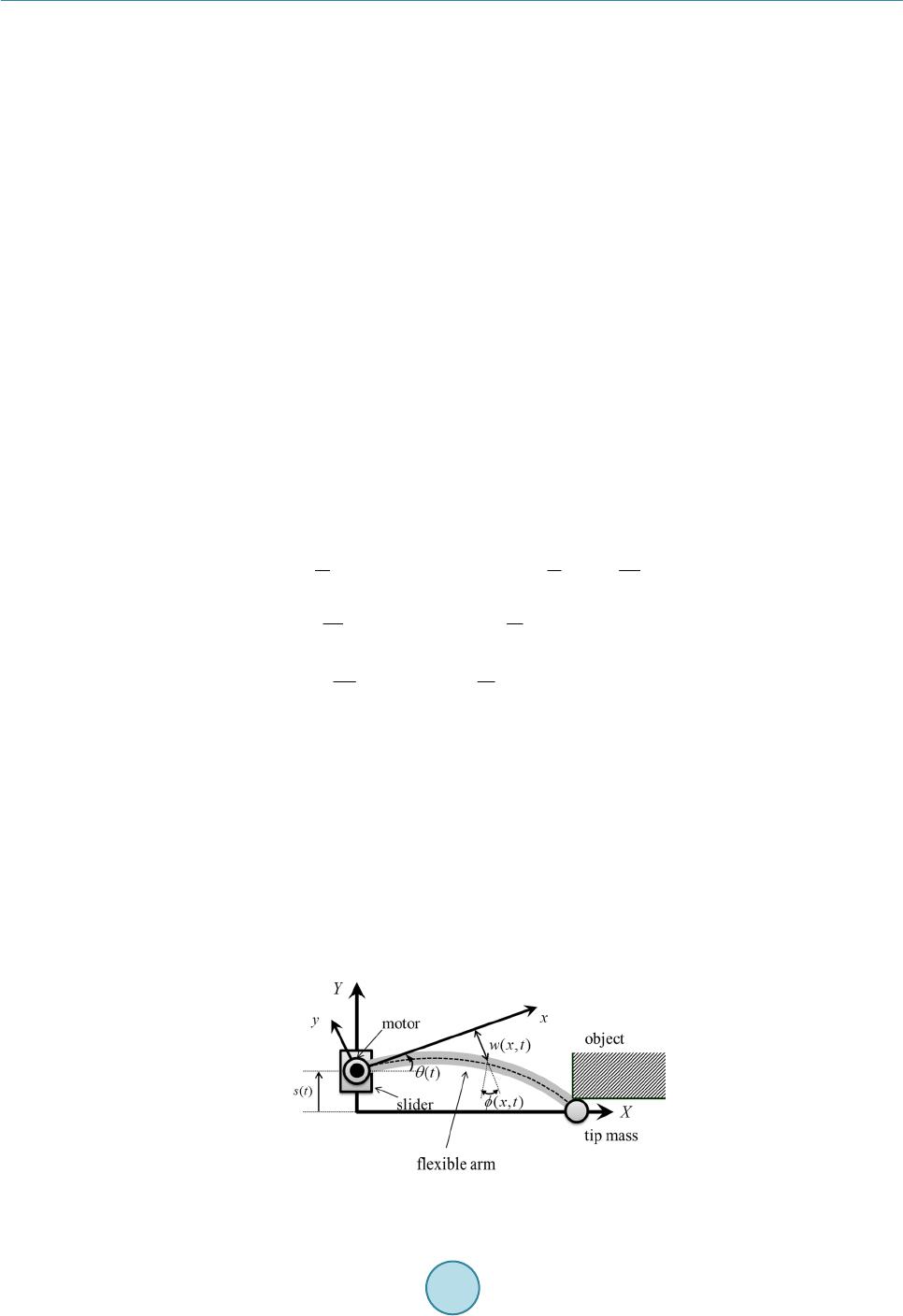

M.Sasakietal.
107
has a wider application area than the Euler-Bernoulli beam theory. So we discuss the force control problem for
the flexible Timoshenko arm.
2.EquationsofMotionandBoundaryConditions
Figure 1 shows a constrained one-link flexible Timoshenko arm. One-end of the arm is clamped to control ac-
tuators consisting of the rotational motor and the translational slider, and the other end has a concentrated tip
mass m. The tip mass makes contact with the surface of an object. The flexible arm translates and rotates in the
horizontal plane (the XY plane in Figure 1) by control actuators; it is not affected by the acceleration of grav-
ity. The flexible arm, with length l, mass per unit length

, mass moment of inertia I

, cross sectional area
A, area moment of inertia
I
, Young’s modulus E, shear modulus G, and shear coefficient

, satisfies the
Timoshenko beam hypothesis.
In Figure 1, XY is an absolute coordinate system and
x
y is a local coordinate system, whose origin is
fixed at the rotor of the rotational motor. In addition,
x
y translates with the slider and rotates with the rotor of
the motor. Let
J
, ()
mt

, ()t

,
M
, ()
s
F
t, and ()
s
t be the inertia moment of the motor, the torque gener-
ated by the motor at time t, the rotational angle of the motor, the mass of the slider, the force generated by the
slider, and the translational position of the slider, respectively. Further, let (,)wxt and (,)
x
t

be the trans-
verse displacement of the flexible arm at time t and spatial point
x
, and the rotation of the cross section due
to bending deformation, respectively.
Since the tip mass makes contact with the surface of the object, we obtain the following geometric constraint:
()(,)() 0lt wlt st


  .
This constraint means that the Y-axis position of the tip mass is constrained on the surface of the object. The
kinetic energy
K
E and the potential energy
P
E of the overall system are given by the following:
22 2
0
22
0
[()(,)()]d()()
222
[()(,)]d[()(,)()],
22
l
K
l
JM
Extwxtstxtst
Im
txtxltwltst



 





 
 
22
00
[(,)]d[(,) (,)]d,
22
ll
PEI K
Extxxtwxtx 
 

where KGA  , a dot denotes the time derivative, and a prime denotes the partial derivative with respect to
x
. Here the virtual work is given by δ() δ()() δ()WttFtst



.
Under the above preparation, we can obtain the following equations of motion by applying Hamilton’s princi-
ple and Lagrange’s multiplier, and using the procedure described in [13]:
[( ,)()()][( ,)( ,)]0,wxtxtstKxtw xt  


 

  (1)
[ (,)()][(,)(,)](,)0,IxttKxtw xtEIxt
 
  
  (2)
(0,)(0, )(, )()(, )()0,wttltlt wlt st




(3)
()()(0,) (),
m
J
ttEItt  
  
 (4)
Figure 1. Flexible Timoshenko arm making contact with an object.

M.Sasakietal.
108
()()(0,) (),
s
M
st FtKwt Ft



 (5)
with the algebraic relation
()[(,)(,)],tKwlt lt



 (6)
where ()t

is Lagrange’s multiplier and is equivalent to the contact force, i.e., the shear force at the tip of the
flexible arm, which arises in the direction along the normal vector of the constraint surface.
The aim of this paper is to control the contact force at the tip of the flexible arm. In other words, the control
objective is to construct a boundary controller satisfying
(), (,)0, (,)0,
()0, ()0,
d
twxt xt
tst
 






 (7)
where d

is the constant desired contact force. At the desired equilibrium point
((), (,)(,)()()0
d
twxtxtt st   


), (,)wxt and (,)
x
t

become the function of the variable
x
, and
()t

and ()
s
t become constant. Thus, we describe them as ()
d
wx , ()
d
x

, d

, and d
s
, respectively. By sub-
stituting these into (1)-(6), we obtain:
2
2
1
(), (),
26 2
1
,
3
d
dd d
dd d
x
lx xx
wx xxl
KEIEI EI
l
ls l
KEI









 

 



(8)
In these relations, ()
d
wx, ()
d
x

, d

, and d
s
mean a static transverse displacement, a static rotation of the
cross section of the flexible arm, a static angle of the motor, and a static position of the slider in the case where
the contact force is converged to the desired value, respectively. Furthermore, d

and d
s
are coupled through
d

, and thus we cannot set the desired angle d

and the desired position d
s
independently.
Based on these results, we set the control objective as follows: to construct a controller accomplishing:
(,)(), (,) 0,
(,)(), (,)0,
(), ()0, (), ()0.
d
d
dd
wxtwxwxt
xtx xt
ttstsst











(9)
For this purpose, we propose the following controller:
1234
( )[(0,)(0)](0,)[( )](),
dd
FtkKwtwkKwtk stskst
 


 (10)
5678
()[ (0,)(0)](0,)[()](),
dd
tkEItkEItk tkt 


  
(11)
where feedback gain i k
, 1,,8i, is a positive constant. In these controllers, (10) is the controller for the
slider and (11) is the controller for the motor. In (10), the first and second terms are for the control:
(,) ()
d
wxtwx and (,) 0wxt
, and the third and the forth terms are for the position control: () d
s
ts and
() 0st
. On the other hand, in (11), the first and second terms are for the control of the rotation of the cross
section: (,) ()
d
x
tx

and (,) 0xt
 
, and the third and the forth terms are for () d
t

  and ()0t
 
.
Here, note that if we use the strain gauge, rotary encoder, and speed reference type servo amplifier of the motor
and the slider, we can easily implement the controller.
3.LaplaceTransformoftheEquationofMotion
Taking the Laplace transform of (1)-(11), we can get














22
,, ,0swxsK xsKwxssxsSs  
  
(12)








22
,, ,0sIKxsKwxsEI xssIs


 
(13)


0, 0ws

(14)

M.Sasakietal.
109


0, 0s 

(15)


,0ls 


(16)






,0ls wls Ss 


(17)




2(0,)( )
m
s
JssEIss 



  (18)






2(0, )
s
s
MS sFsKwsF s

  (19)




 
12341 3
1
0,(0 )
dd
F
skskKw'skskSsk Kw'kS
s
 
 (20)




 
567857
1
0,(0 )
dd
skskEIsksksk EIk
s


   


(21)
Finally we get


0,ws
and


0,
s

as follows:


 



 


22 2
4378
22
4378
2222222 2
32
84 263487
22
348716253847
11
0,( 221
4
*(
1
*(4 2
(2
11
222
ws FsFs
KsskskksksE I
sksk ksks
sEIKEsIKIKsI sEIIK
kkEIIKsEKkkkkkkI
I KkJkkMksEkkkkKkkkk








 

 


 

 





 
2
38 47371537
2222222 2
22
4378
2222222 2
32
84 2
1
)2() ))
2
1
*4
2
2
1
*4
2
(2
I
KIkkkksEkkKkkIKI kk
KEIsEIKsIsEIKEsIKIKs Is
sk s kk sks
sEIKEsIKIKsI sEIIK
kkEIIKsEKk











 


 














   


63487
22
3487162538 47
2
38 47371537
2 2
1278
2222222 2
127
11
222
1
)2() ))
2
2(32 1 4*
1
42
kkkkkI
IKkkkk sEkkkk KkkkkI
KIkkkksEkkKkkIKI kk
EIKsFsFsF sFskskksks
sEI KEsIKIKsI
sk skk






 

 


 
 




 




  


  
222
8
2
1325 7
81 3125771 3
*2
*12342( (
)))0,
ddd d
ddd ddd
sksEIIKsK
F
sFsFsFskkSskklk K
kk kSskkklkKkk kSK




 

(22)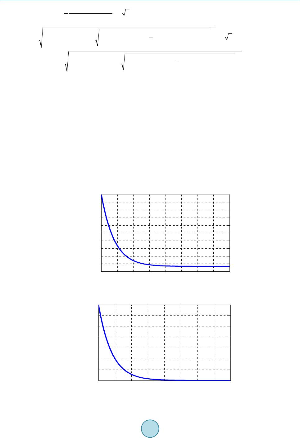

M.Sasakietal.
110


   
  

 
56
2
78
2222222 2
2222222 2
56
57
11
0,( 221
2
1
*4 243
2
1
*4
2
2()) 123
dd
ssFsFsksk
Ks ksks
K
EIsEIKsIsEIKEsIKIKsIssFs Fs
k skKEIsEIKsIsEIKEsIKIKsIs
Kkl kF sFsF






 



  






 





 
40,sFs
(23)
where the constants






1,2,3 and4()FsFsFsFs can be determined using the boundary conditions.
4.NumericalSimulationResults
Numerical inversion of Laplace transform is used to obtain the results in the time domain. The computation of
the inverse Laplace transform is based on the paper of T. Hosono [12]. In the computer simulation study, we
consider a typical arm whose parameters are given in the Table 1. To investigate the validity of the proposed
controller, we considered the step responses of the desired contact force, 100
d


 N, and the desired posi-
tion of the slider, 0.1
d
s m. Here, note that 100
d


 means that the flexible arm pushed the surface of the
environment by the force of 100 N. Figures 2-6 show the time response of the transverse displacement, the an-
gle of deflection, the slider position, the rotational angle and the contact force with adequate feedback gains
15
1kk , 26 0.2kk , 37 16kk, 48 8kk

 using try and error method. The desired value of d w,
d

, d

are
00.25 0.5 0.7511.25 1.5 1.752
-5
-4.5
-4
-3.5
-3
-2.5
-2
-1.5
-1
-0.5
0x 10
-3
w[m]
t[s]
Figure 2. Time response of transverse displacement of the arm.
00.25 0.50.7511.25 1.5 1.752
-7
-6
-5
-4
-3
-2
-1
0x 10
-3
t[s]
φ[rad]
Figure 3. Time response of angle of deflection of the arm.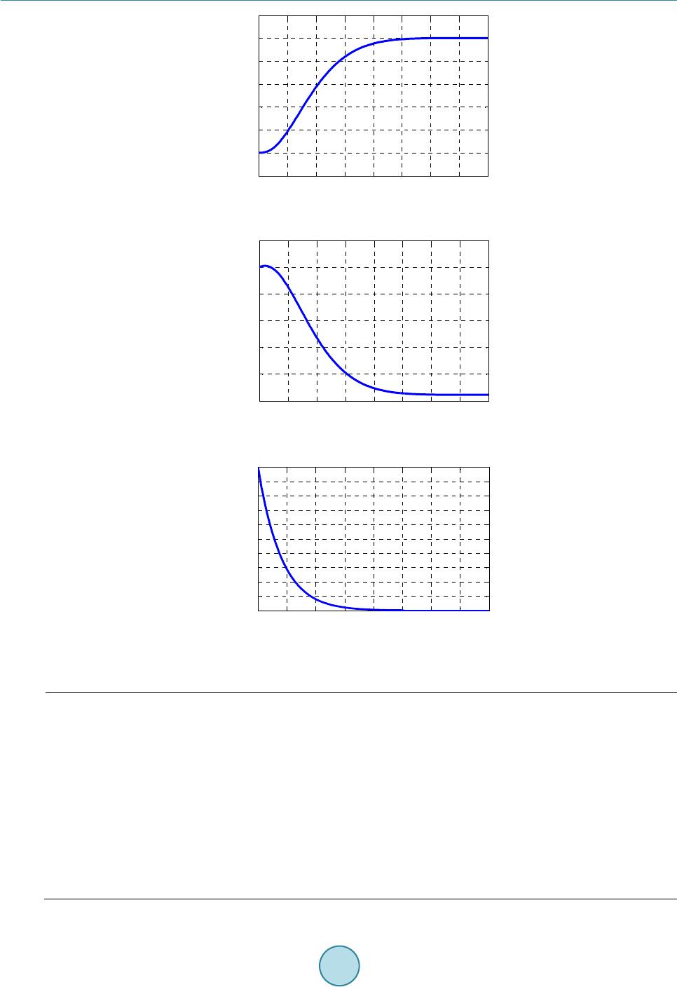

M.Sasakietal.
111
00.25 0.5 0.75 11.25 1.5 1.752
-0.02
0
0.02
0.04
0.06
0.08
0.1
0.12
t[s]
S[m]
Figure 4. Time response of the slider position.
00.25 0.5 0.75 11.251.5 1.75 2
-0.1
-0.08
-0.06
-0.04
-0.02
0
0.02
t[s]
θ[rad]
Figure 5. Time response of rotational angle.
00.25 0.5 0.7511.25 1.5 1.752
-100
-90
-80
-70
-60
-50
-40
-30
-20
-10
0
t[s]
λ[ N ]
Figure 6. Time response of the contact force.
Table 1. System parameters.
Length l 1.0 [m]
Mass per unit length

2.73 [kg/m]
Mass moment of inertia
I

2.79e (−4) [kgm]
Cross sectional area A 3.5e (−4) [m4]
Area moment of inertia
I
3.57e (−8) [m4]
Young’s modulus E 2.00e11 [Pa]
Shear modulus G 7.69e10 [Pa]
Shear coefficient

5/6
Desired contact force d

−100 [N]
Desired translational position of the slider d
S 0.1 [m]

M.Sasakietal.
112



3
3
7.00 10[]
4.67 10 []
0.0953[ ]
d
d
d
x
rad
wx m
rad





 



(24)
It can be seen that the transverse displacement, the angle of deflection, the slider position, the rotational angle
and the contact force toward the desired their values. With the adequate feedback gains there are no residual vi-
brations and no over shoot.
5.Conclusion
A contact-force control problem with regards to a constrained one-link flexible Timoshenko arm was described.
The equations of motion and the boundary conditions of the overall system were derived. To solve the contact
force control problem of such a system, we have proposed a simple controller, which is easy to implement. Sev-
eral numerical simulations using a numerical inversion of Laplace transform were carried out. The simulation
results showed the validity of the proposed controller for the contact-force control problem with no residual vi-
brations and no overshoot.
References
[1] Yuan, K. and Hu, C.-M. (1996) Nonlinear Modeling and Partial Linearizing Control of a Slewing Timoshenko-Beam.
Trans. ASME Journal of Dynamic Systems, Measurement, and Control, 118, 75-83.
http://dx.doi.org/10.1115/1.2801154
[2] Tadi, M. (1997) Comparison of Two Finite-Element Schemes for Feedback Control of a Timoshenko Beam. Proceed-
ings of the ASME Dynamic Systems and Control Division, 61, 587-596.
[3] White, M.H.D. and Heppler, G.R. (1996) Vibration of a Rotating Timoshenko Beam. Trans. ASME Journal of Vibra-
tion and Acoustic, 118, 606-613. http://dx.doi.org/10.1115/1.2888341
[4] Sasaki, M., Ueda, T., Inoue, Y. and Book, W.J. (2012) Passivity-Based Control of Rotational and Translational Ti-
moshenko Arms. Advances in Acoustics and Vibration, 2012, Article ID: 174816.
http://dx.doi.org/10.1155/2012/174816
[5] Morgül, Ö. (1992) Dynamic Boundary Control of the Timoshenko Beam. Automatica, 28, 1255-1260.
http://dx.doi.org/10.1016/0005-1098(92)90070-V
[6] Oguamanam, D.C.D. and Heppler, G.R. (1996) The Effect of Rotating Speed on the Flexural Vibration of a Ti-
moshenko Beam. Proc. of the 1996 IEEE International Conference on Robotics and Automation, 2438-2443.
http://dx.doi.org/10.1109/ROBOT.1996.506529
[7] Zhang, F., Dawson, D.M., de Queiroz, M.S. and Vedagarbha, P. (1997) Boundary Control of the Timoshenko Beam
with Free-End Mass/Inertial Dynamics. Proc. of the 36th IEEE Conference on Decision & Control, 245-250.
http://dx.doi.org/10.1109/CDC.1997.650623
[8] Taylor, S.W. and Yau, S.C.B. (2003) Boundary Control of a Rotating Timoshenko Beam. ANZIAM J., 44, E143-E184.
[9] Rastgoftar, H., Mahmoodi, M., Eghtesad, M. and Kazemi, M. (2008) Stability Analysis of a Flexible Two-Link Ti-
moshenko Manipulator Using Boundary Control Method. Proc. of ASME 2008 International Mechanical Engineering
Congress and Exposition, 409-415.
[10] Grobbelaar-Van Dalsen, M. (2010) Uniform Stability for the Timoshenko Beam with Tip Load. J. Math. Anal. Appl.,
361, 392-400. http://dx.doi.org/10.1016/j.jmaa.2009.06.059
[11] Han, Z.J. and Xu, G.Q. (2011) Dynamical Behavior of a Hybrid System of Nonhomogeneous Timoshenko Beam with
Partial Non-Collocated Inputs. J. Dyn. Control Syst., 17, 77-121. http://dx.doi.org/10.1007/s10883-011-9111-6
[12] Hosono, T. (1981) Numerical Inversion of Laplace Transform and Some Application to Wave Optics. Radio Science,
16, 1015. http://dx.doi.org/10.1029/RS016i006p01015
[13] Endo, T., Matsuno, F. and Kawasaki, H. (2014) Force Control and Exponential Stabilisation of One-Link Flexible Arm.
Int. J. Control, 87, 1794-1807. http://dx.doi.org/10.1080/00207179.2014.889854