Received 11 August 2015; accepted 15 October 2015; published 22 October 2015

ABSTRACT

Let C be a set of colors, and let be an integer cost assigned to a color c in C. An edge-coloring of a graph is assigning a color in C to each edge so that any two edges having end-vertex in common have different colors. The cost of an edge-coloring f of G is the sum of costs of colors assigned to all edges e in G. An edge-coloring f of G is optimal if is minimum among all edge-colorings of G. A cactus is a connected graph in which every block is either an edge or a cycle. In this paper, we give an algorithm to find an optimal edge- coloring of a cactus in polynomial time. In our best knowledge, this is the first polynomial-time algorithm to find an optimal edge-coloring of a cactus.

Keywords:

Cactus, Cost Edge-Coloring, Minimum Cost Maximum Flow Problem

1. Introduction

Let be a graph with vertex set V and edge set E, and let C be a set of colors. An edge-coloring of G is to color all the edges in E so that any two adjacent edges are colored with different colors in C. The minimum number of colors required for edge-colorings of G is called the chromatic index, and is denoted by. It is well-known that 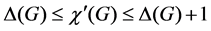for every simple graph G and that for every bipartite (multi)graph G, where is the maximum degree of G [1]. The ordinary edge-coloring problem is to compute the chromatic index of a given graph G and find an edge-coloring of G using colors. Let be a cost function which assigns an integer to each color, then the cost

edge-coloring problem is to find an optimal edge-coloring of G, that is, an edge-coloring f such that

is minimum among all edge-colorings of G. An optimal edge-coloring does not always use the minimum number of colors. For example, suppose that and for each index, then the graph G with in Figure 1(a) can be uniquely colored with the three cheapest colors, and as in Figure 1(a), but this edge-coloring is not optimal; an optimal edge-coloring of G uses the four cheapest colors, , and, as illustrated in Figure 1(b). However, every simple graph G has an edge-coloring

using or colors [2] [3]. The edge-chromatic sum problem, introduced by Giaro and Kubale [4], is merely the cost edge-coloring problem for the special case where for each integer.

The cost edge-coloring problem has a natural application for scheduling [5]. Consider the scheduling of biprocessor tasks of unit execution time on dedicated machines. An example of such tasks is the file transfer problem in a computer network in which each file engages two corresponding nodes, sender and receiver, simultaneously [6]. Another example is the biprocessor diagnostic problem in which links execute concurrently the same test for a fault tolerant multiprocessor system [7]. These problems can be modeled by a graph G in which machines correspond to the vertices and tasks correspond to the edges. An edge-coloring of G cor- responds to a schedule, where the edges colored with color represent the collection of tasks that are executed in the ith time slot. Suppose that a task executed in the ith time slot takes the cost. Then the goal is to find a schedule that minimizes the total cost, and hence this corresponds to the cost edge-coloring problem.

The cost edge-coloring problem is APX-hard even for bipartite graphs [8], and hence there is no polynomial- time approximation scheme (PTAS) for the problem unless. On the other hand, Zhou and Nishizeki gave an algorithm to solve the cost edge-coloring problem for trees T in time, where n is the number of vertices in T, is the maximum degree of T, and is the maximum absolute cost of colors c in C [5]. The algorithm is based on a dynamic programming (DP) approach, and computes a DP table for each vertex of a given tree T from the leaves to the root of T. In this paper, we give a polynomial-time algorithm to solve the cost edge-coloring problem for cacti. In our best knowledge, this is the first polynomial- time algorithm to find an optimal edge-coloring of a cactus.

2. Preliminaries

In this section, we define some basic terms.

Let be a graph with a set V of vertices and a set E of edges. We sometimes denote by and the vertex set and the edge set of G, respectively. We denote by and, respectively, or simply by n and m, the number of vertices and edges in G, that is, and. The degree of a vertex v is the number of edges in E incident to v. We denote the maximum degree of G by or simply by. A cactus G can be represented by an under tree T, which is a rooted tree. In the underlay tree T of G, each node represents a block which is either a bridge (edge) of G or an elementary cycle of G. If there is an edge between nodes and of T, then bridges or cycles of G represented by and share exactly one vertex in G. Each node b of T corresponds to a subgraph of G induced by all bridges and cycles represented by the nodes that are descendants of b in T. Figure 2(a) depicts the subgraph for the child of the root r of T. Clearly and is a cactus for each node b of T. One can easily find an underlay tree T of a given cactus G in linear time, and hence one may assume that an underlay tree of G is given. We denote by the number of edges joining a node b and its children in T. Then, , and for every vertex.

Let C be a set of colors. An edge-coloring of a graph G is to color all edges of G by colors in C so that any two adjacent edges are colored with different colors. Let, where is the set of real numbers. One may assume with loss of generality that is non-decreasing, that is, for any

index i,. Since trivially any graph G has an optimal edge-coloring using colors at most, we assume for the sake of convenience that, and we write. The cost of an edge-coloring f of a graph is defined as follows:

An edge-coloring f of G is called an optimal one if is minimum among all edge-colorings of G. The cost edge-coloring problem is to find an optimal edge-coloring of a given graph G. The cost of an optimal edge-coloring of G is called the minimum cost of G, and is denoted by.

Let f be an edge-coloring of a graph G. For each vertex v of G, let be the set of all colors that are assigned to edges incident to v, that is,

We say that a color is missing at v if. Let be the set of all colors missing at v, that is,.

3. Algorithm

In this section we prove the following theorem.

Theorem 1. An optimal edge-coloring of a cactus can be found in polynomial time.

As a proof of Theorem 1, we give a dynamic programming algorithm in the remainder of this section to compute the minimum cost of a given cactus G. Our algorithm can be easily modified so that it actually finds an optimal edge-coloring f of G with.

A dynamic programming method is a standard one to solve a combinatorial problem on graphs with tree- construction. We also use it, and compute the minimum cost of a cactus G with an under tree T by the bottom-up tree computation.

3.1. Ideas and Definitions

Let b be a node of T with its parent, and let v be the vertex on both two blocks b and. Let be the children of b in T. Then one can observe that the minimum cost of the subgraph rooted at b cannot be computed directly from the minimum costs of all the subgraphs,. Our idea is to introduce a new parameter defined for each node b of T and each pair of colors as follows:

If has no such edge-coloring we define. Note that if either the block b is an edge and or the block b is a cycle and. Clearly,

We compute the values for all indices, , from leaves to root r. Thus the DP table for each node b consists of the values,.

Our algorithm computes for all pairs of colors from the leaves to the root r of T, by means of dynamic programming. Then can be computed at the root r from all the values as follows:

and it can be computed in polynomial time. Thus the remainder problem is how to compute all the values for each node of T and all pairs of colors.

3.2. Algorithm

In this subsection, we explain how to compute all the values for each node of T and all pairs of colors.

3.2.1. The Node b Is a Leaf in T

In this case, the block b is either an edge or a cycle. Therefore we have the following two cases to consider.

Case 1: the block b is an edge.

In this case, clearly

and all the values, , can be computed in time polynomial in.

Case 2: the block b is a cycle.

In this case, we describe the following algorithm to compute in time polynomial in the size of and.

3.2.2. The Node b Is an Internal Node

In order to compute for each pair of indices and, , we introduce a new parameter defined as follows.

Let be a set of blocks of T such that all these blocks share exactly one vertex v in G. For each pair of colors we define

We show how to compute the all the values from the values, and. The problem of computing can be reduced to the minimum cost flow problem on a bipartite graph as follows.

We first introduce isolated vertices, and. Then add vertices, , corresponding to colors, and add a source s and a sink t. Connect the source s to all the vertices, , with capacity 1 and cost 0. For each vertex, and, connect to all the vertices, and, satisfying or with capacity 1 and cost 0. Finally, for each vertex, and, connect to the sink t with capacity 2 and cost. The minimum cost flow problem is to find a maximum flow from s to t with the sum of costs of edges on the flow. Clearly is equal to the cost of the minimum cost maximum flow in.

The minimum cost maximum flow problem can be solved in time polynomial in the size of the graph [9] [10], and hence the value for a pair of indices and, , can be computed in time polynomial in and since has at most vertices and edges. Therefore the values for all pairs of indices and, , can be computed total in time polynomial in and.

We are now ready to compute. Since the block b is either an edge or a cycle, we have the following two cases to consider.

Case 1: the block b is an edge.

Let be the set of blocks of the children of b in T. Then all the blocks share exactly one vertex v in G. In this case, clearly

and it can be computed in time polynomial in the size of and.

Case 2: the block b is a cycle.

In this case, let be the vertices lied on the cycle of in the clockwise order. Assume that is the vertex shared by the block b and its parent block, and let, , be the set of blocks which shares; if no such blocks exist. In order to compute we define

(1)

for each j, , where. Then clearly

Therefore it suffices to show how to compute in polynomial time for each j, , as follows.

By Equation (1) we have

and hence for all j, , can be recursively computed total in time if all the values, , are given. Since we have mentioned before that all the values can be computed in time polynomial in and, one can compute all and hence total in time polynomial in and.

4. Conclusion

In this paper, we show that the cost edge-coloring problem for a cactus G can be solved in polynomial time. It is still open to solve the problem in polynomial time for outerplanar graphs.

Supported

This work is partially supported by grants of the thousand talent plan of Zhejiang province.

Cite this paper

Zhiqian Ye,Yiming Li,Huiqiang Lu,Xiao Zhou, (2015) Cost Edge-Coloring of a Cactus. World Journal of Engineering and Technology,03,119-134. doi: 10.4236/wjet.2015.33C018

References

- 1. West, D.B. (2000) Introduction to Graph Theory. 2nd Edition, Prentice Hall, New Jersey.
- 2. Hajiabolhassan, H., Mehrabadi, M.L. and Tusserkani, R. (2000) Minimal Coloring and Strength of Graphs. Discrete Mathematics, 215, 265-270. http://dx.doi.org/10.1016/S0012-365X(99)00319-2
- 3. Mitchem, J., Morriss, P. and Schmeichel, E. (1997) On the Cost Chromatic Number of Outerplanar, Planar, and Line Graphs. Discussiones Mathematicae Graph Theory, 17, 229-241. http://dx.doi.org/10.7151/dmgt.1050
- 4. Giaro, K. and Kubale, M. (2000) Edge-Chromatic Sum of Trees and Bounded Cyclicity Graphs. Information Process- ing Letters, 75, 65-69. http://dx.doi.org/10.1016/S0020-0190(00)00072-7
- 5. Zhou, X. and Nishizeki, T. (2004) Algorithm for the Cost Edge-Coloring of Trees. J. Combinatorial Optimization, 8, 97-108. http://dx.doi.org/10.1023/B:JOCO.0000021940.40066.0c
- 6. Coffman, E.G., Garey, M.R., Johnson, D.S. and LaPaugh, A.S. (1985) Scheduling File Transfers. SIAM J. Computing, 14, 744-780. http://dx.doi.org/10.1137/0214054
- 7. Krawczyk, H. and Kubale, M. (1985) An Approximation Algorithm for Diagnostic Test Scheduling in Multicomputer Systems. IEEE Trans. Computers, 34, 869-872. http://dx.doi.org/10.1109/TC.1985.1676647
- 8. Marx, D. (2009) Complexity Results for Minimum Sum Edge Co-loring. Discrete Applied Mathematics, 157, 1034- 1045. http://dx.doi.org/10.1016/j.dam.2008.04.002
- 9. Goldberg, A.V. and Tarjan, R.E. (1987) Solving Minimum Cost Flow Problems by Successive Approximation. Proc. 19th ACM Symposium on the Theory of Computing, 7-18. http://dx.doi.org/10.1145/28395.28397
- 10. Goldberg, A.V. and Tar-jan, R.E. (1989) Finding Minimum-Cost Circulations by Canceling Negative Cycles. J. ACM, 36, 873-886. http://dx.doi.org/10.1145/76359.76368