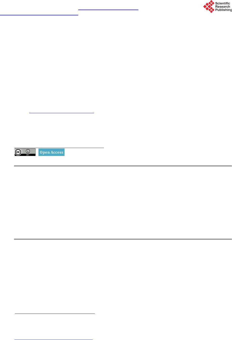
 Journal of Modern Physics, 2015, 6, 1701-1710 Published Online September 2015 in SciRes. http://www.scirp.org/journal/jmp http://dx.doi.org/10.4236/jmp.2015.611172 How to cite this paper: Velázquez, G.L. and Cabrera, G.M. (2015) Study of Decoherence of Entangled States Made up of Two Basic States in a Linear Chain of Three Qubits. Journal of Modern Physics, 6, 1701-1710. http://dx.doi.org/10.4236/jmp.2015.611172 Study of Decoherence of Entangled States Made up of Two Basic States in a Linear Chain of Three Qubits Gustavo López Velázquez*, Gustavo Montes Cabrera Departamento de Física, Universidad de Guadalajara, Blvd. Marcelino García Barragan y Calzada Olímpica, Guadalajara, Mexico Email: *gulopez@udgserv.cencar.udg.mx Received 27 May 2015; accepted 26 September 2015; published 29 September 2015 Copyright © 2015 by authors and Scientific Research Publishing Inc. This work is licensed under the Creative Commons Attribution International License (CC BY). http://creativecommons.org/licenses/by/4.0/ Abstract Using Lindblad approach to study decoherence of quantum systems, we study the decoherence and decay of entangled states, formed by two basic states of a chain of thee qubits. We look on these states for a possible regular dependence on their decay as a function of their energy separa- tion between the basic states under different types of environments. We didn’t find regular or sig- nificant dependence on this energy separation for the type of environment considered. Keywords Decoherence, Entangled States, Three Quits, Linear Chain 1. Introduction In the real world (quantum or classical) the interaction of the system with the environment is unavoidable. In pri nciple, o ne could study t he unitar y evo lution o f the whol e syste m, qua ntum p lus envir onme nt plus qua ntum- environment interaction, but this represents a many-bodies problem which is unsolvable within any picture of the quantum mechanics. The most used ap proach t o study this phenomenon is to use the matrix density approach for the whole system and to make the trace over the environment variables [1]-[5]. The re sultin g densi ty matr ix is called “reduced density matrix”, and its associated non-unitary evolution equa tion is call ed “master eq uation”. This equation is pheno menological where dissipati ve and diffusion parameters are de fined, and they are respon- sible of the decay behavior of the non diagonal elements of the reduced density matrix. This phenomenon is *  G. L. Velázquez, G. M. Cabrera called “decoherence” because it is related with the disappearance of the interference in terms of the product of the quantum wave function [6] [7] and many think that this decoherence effect is closely related with the ap- pearance of the classical world [7]-[9]. In most of the approaches, the positiveness and trace equal to one are kept as principal condition for the reduced density matrix. The best known mathematical approach which kept these c ond ition s was gi ven b y Lind blad [10], which ga ve an abstr act ge neral non u nitar y evol ution e quat ion fo r the reduced density matrix. The master equation is different when dealing with continuous systems (quantum Browning motion, for example) [1] [2] or discrete quantum systems (spin system) [11]. One of the used ap- proaches for quantum discrete system is described in [12], and we will use this approach for our study of deco- herence of entangled states built up with two states of three qubits in a quantum computer model of a linear chain of three paramagnetic atoms with nuclear spin one half [13]. In this work, we are interested in determining the decoherence of several entangled states formed by two states of three qubits, and we will use the above men- tioned Markovian-Lind b lad master type of equation [4] [12]. O n the ot her hand , even this model for sol id state quantum computer has not been built; it has been very useful for theoretical studies about implementation of quantum gates and quantum algorithms [13]-[16] which can be extrapolated to other solid state quantum com- puters. The main idea is to explore the possible sensitivity of the decay of an entangled state with respect to the energy-difference of its two sta tes involved; we establish four cases to be considered with the quantum-environ- ment system: indep endent env ironment interactio n, pure dephasing interactio n, cor related dissipatio n interaction, and dephasing correlated interaction. The analytical dynamical systems of the reduced density matrix elements are obtained for these cases, and the results of the analytical and numerical simulations are presented. 2. Hamiltonian of the Chain of Nuclear Spins Follo wing Llo yd’s idea [17], consider a linear chain of nuclear spin one half, separated by some distance and in- side a magnetic in a direction z, , and making and angle with respect this linear chain. Choosin g this angle such that , the dipole-dipole interaction is canceled, the Larmore’s fr equenc y for each spin is different, with th e g yro mag netic ratio. The magnetic moment of the nucleus is related with its spin through t he r e la tion , and the interaction energy between the magnetic field and magnetic moments is ( ) z intkkk k kk HBz S ω =−⋅=− ∑∑ µ . If in addition, one has first and second neighbor Ising interact ion, the Hamiltonian of the system is just [13] 12 12 11 1 22 , NN N z zzzz s kkkkkk kk k JJ HS SSSS ω −− ++ = == ′ =−−− ∑∑ ∑ (1) where N is the number of nuclear spins in the chain (or qubits), J and J' ar e the c oup ling c onst ant o f the nucl eus at first and second neighbor. Using the basis of the register of N-qubits, with , one has that . Therefore, the Hamiltonian is diagonal on this basis, and its eigenvalues are ( )( )( ) 12 12 11 1 1 11. 22 2 kkk kk NN N k kk k JJ E ξξξ ξξ ξ ω ++ −− ++ = == ′ =−− −−−− ∑∑ ∑ (2) 3. Interaction with the Environment Consider now that the environment is characterized by a Hamiltonian and its interactin g with the quantum system with Hamiltonian . Thus, the total Hamiltonian would be , where is the part of the Hamiltonian which takes into account the interaction system-environment, and the equation one would need to so lve, in terms of the density matrix, is [18] [19] (3) where is the density matrix which depends on the system and environment coordinates. The evo- lution of the system is unitary, but it is not possible to solve this equation. Therefore, under some approxima- tions and traci ng over the envi ronment c oordinates [5] [20], it is possible to a rrive to a Lindblad type of equatio n [4] [21] for the reduced density matrix ,  G. L. Velázquez, G. M. Cabrera [ ] † †† 1 11 ,22 I siii iii i iHVVV VVV t ρρ ρρρ = ∂ =+−− ∂ ∑ (4) where are called Kraus’ operators. This equation is not unitary and Markovian (without memory of the dy- namic al p roc ess) . T his eq uati on c an be writ te n in t he i nter ac tio n pict ure, thr ou gh the tra nsfo r matio n with , as (5) where is the Lindblad operator ( ) † †† 1 11 22 I iii iii i VVV VVV ρ ρρρ = = −− ∑ (6) with . The explicit form of Lindblad operator is determined by the type of environment to consider [12] at zero temperature. In this work we consider dissipation effects and dephasing. So, the operators can be (for dissipation), (for dephasing), and is the coupling constant with the environment. In this way, one considers the following cases: 1) Independent: In this case, each qubit of the chain acts independently with the environment, and one has local decoherence of the system. The Lindblad operator is ( ) ( ) 12 2 N kk kkkkk k S SSSSS i ργ ρρρ − ++−+− = −− ∑ (7) where and are the ascend and descend operators such that ˆ † e, k it kk k SUS US ±Ω ±± ± = = (8) where has been defined as ()( ) 112 2 ˆ. zzz z kkkkkk JJ w SSSS +−+ − ′ Ω= ++++ (9) 2) Correlated independent: Each qubit interact with the environment but its effect is felt by the other qubits, that is, the type of interaction is nonlocal with a collective interction between qubits and environment. The Lindblad operator is ( ) ( ) , 12 2 Njk k jjkjk jk S SSSSS i γ ρρ ρρ − ++−+− = −− ∑ (10) where are t he co upling co nstant between qubits and environment, with and . 3) Dephasing: There is not interchange o f energy bet ween qubits a nd environme nt, only decoherence is pre- sented where the non diagonal ele ments of the reduced density matrix go to zero. The Lindblad operator is ( ) ( ) 12 Nz zzzzz kkkkkkk k S SSSSS i ρρ ρρ =Γ −− ∑ (11) where is the parameter of the kth-qubit which take into account the dephasing of the qubit with the envi- ronment (the tilde operators do not appear due to commutation of this operators with the evolution operator U). 4) Correlated dephasing: Here, one takes into account the collective effect of the environment to the qubits. Lindblad’s operator is of the form ( ) ( ) , 12, Nz zzzzz jkkjjkjk jk S SSSSS i ρρ ρρ =Γ −− ∑ (12) where is the parameter with take into account the correlation . The analytical solutions for these four c ases are given in the Appendix.  G. L. Velázquez, G. M. Cabrera 4. Entanglement and GME-Concurrence Our 3-qubits Hilbert space H is generated by the basis . Labeling the qubit of the 3-qubits chain as ABC, we understand an entanglement of the form AB when the qubits are entangled, and we under- stand an e ntanglement of the f orm ABC when the 3-qubits are entangled. The entangled state under our consideration are listed on Table 1 . We chose these state since they are mostly used on experiments of quantum computation or quantum information. Table 1. Entangled states ( ordered according t heir en er gy separation ). Entangled form Initial entangled state ABC AB BC AC In order to quantify the entanglement of a state formed by three qubits basis-states, we will use the criteria given on [22]-[24] where the lower bound of the concurr ence is () { } 22 GME 1, , 2 N C ββ β ρρ ⊗⊗ Φ ≥ΦΠΦ −ΦΠΠΦ ∑ (13) where is a separable state of the two copies of the Hilbert space, . is the permutation op er- ator acting on the double copies of the Hilbert space, , inte r c han gi ng e l e me nt s o f one sp ac e i nto the ot h- er, for example { } ( ) 121 2121 2 1 φφψψψ φφψ Π ⊗=⊗ . if , acting on means that the qubit label by “l” is fixed and the qubits label “m” and “n” are interchanged ( , ). Denoting by , one has the fallowing GME-concurrence associated to the given entangled state (Tab l e 2):  G. L. Velázquez, G. M. Cabrera Table 2. Entanglement form: ABC. State GME-concurrence 1844 5533 662277 22 2 2 ρ ρρ ρρ ρρ −−− 271188336644 55 22 22 ρρρρρ ρρ −−− 3611 8822 7744 55 22 22 ρρρρρ ρρ −−− 4511 8822773366 22 22 ρρρ ρρ ρρ −−− For the case when entangled state is of the form AB, BC or AC, one makes the trace on the missing letter qubit, and it follows that (Table s 3-5) GME 2 ABAB AB Cil kjijijkl kl ρ ρρ = − (14) Table 3. Entanglemet form: AB. State GME-concurrence ( )( ) 172833 44 55 66 22 ρρ ρρρρ +− ++ ( )() 35 4611 22 77 88 22 ρρρρρρ +− ++ Table 4. Entanglement form: BC. State GME-concurrence ( )( ) 14 5822 66 33 77 22 ρρ ρρρρ +− ++ ( )() 23 671155 44 88 22 ρρρρρρ +− ++ Table 5. Entanglement form: AC. State GME-concurrence ( )( ) 16 382244 55 77 22 ρρ ρρρρ +− ++ ( )() 23471133 6688 22 ρρρρρρ +− ++ 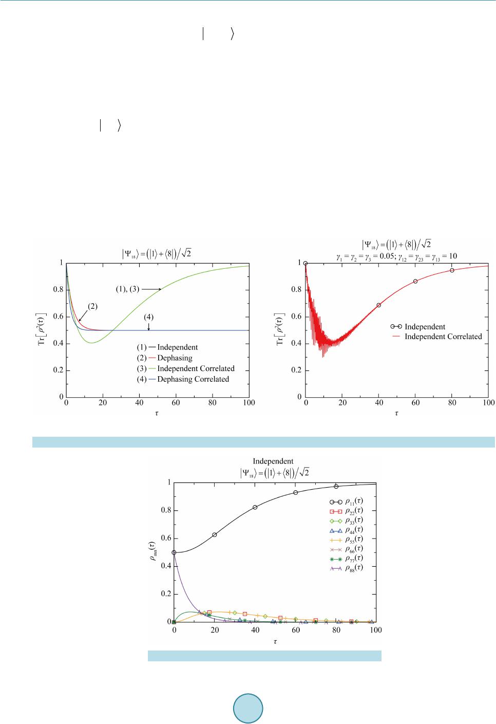 G. L. Velázquez, G. M. Cabrera 5. Results In our case, we have three qubits space , and our parameter in units 2π MHz are 123 123 123 12 2313122313 400;200;100;10;0.4 0.05; 0.05; 0.05;0.05;0.05;0.05 0.05;0.025 0.0125;0.05;0.025;0.0125 JJ ωωω γγγ γγ γ ′ ==== = === Γ= Γ= Γ= ===Γ= Γ=Γ= the time is normalized by the same factor of 2π MHz. To determine the departure of the pure state entangled state, we use the purity parameter, [25]. Figure 1(a) shows the behavior of this parameter for the entangled state as a function of time, where one can see that correlations does not affect much t he ind e- pendent model of the environment, which can be seen only for much bigger dissipation parameters, Figure 1(b). Dephasing models finish with the mix state on the system a t the end, instead of a pure state of the independent model. As seen on Figure 2, ind epend ent mo del end s wit h a p ure stat e in t he s ystem d ue to the s ystem end s on the ground state after sharing energy with the environment. Let us see now how the GME-conc urrenc e and Purit y beha ve for different entangled state and different envi- ronments. Independent Model: For the entangled states listed on Table 1, Figure 3(a), Figure 3 (c) , Figure 4(a ), and Figure 4(c) show GME-concurrence, and Figure 3(b), Figure 3(d), Figure 4(b), and Figure 4(d) show their (a) (b) Figure 1 . Independent model: (a) Purity behavior with 4-models environments; (b) Indepent model with big dissipation. Figure 2 . Diagonal matrix elements behavior. 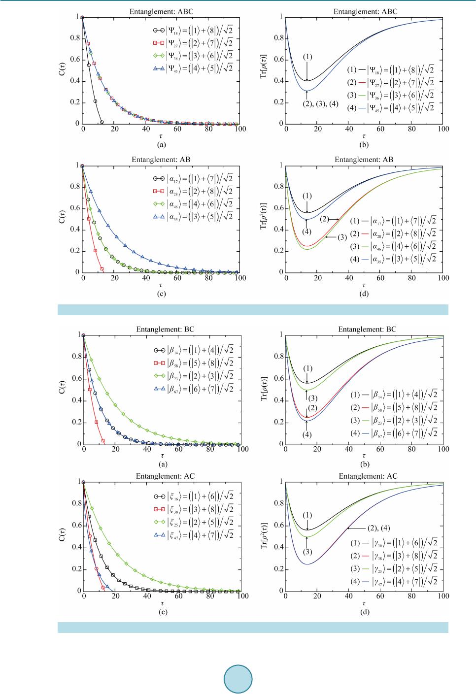 G. L. Velázquez, G. M. Cabrera Figure 3 . Independent: (a), (c) GME-concurrence vs τ . (b), (d) Purity vs τ . Figure 4. Independent: (a), (c) GME-concurrence vs τ . (b), (d) Purity vs τ . 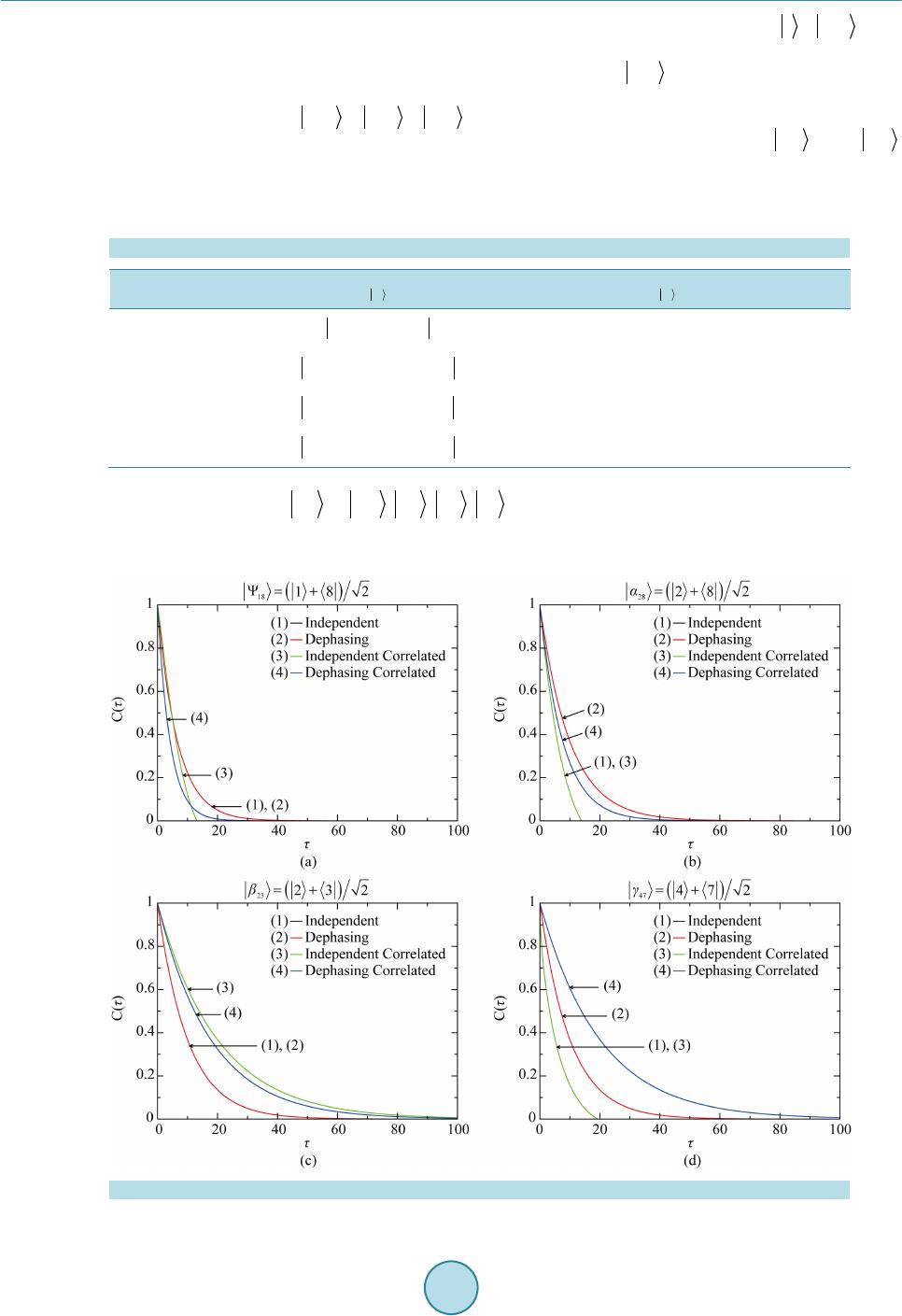 G. L. Velázquez, G. M. Cabrera associated Purity parameter behavior. The system always finish on the pure ground states , the lowest bound of the GME-conc urrenc e fall d own ( altho ugh this parameter can not tell us whether or not the en- tanglement has been completely destroyed). Except for the entangled state (maximum entergy difference between their entangled qubits), there is not clear difference how this entanglement decay is developed. For example, the entangled states , , have the same GME-concurrence decay behavior, but these states have different energy-difference on their associated qubits. The entangled states and the GME-concurrence decay is the same, although their energy-differe nce is q uite big. Dephasing model: In this case, the GME-concurrence and purity parameters can be expressed explicitly in a simple form as shown in Table 6 : Table 6. Exact solution for dephasing model. Entanglement (ABC) , ( )( )( )() 22 2 0020 exp ii jjij ρρ ρτ + +−Γ (AB) ( )() 12 20exp ij ρτ − Γ +Γ , ( )( )()() 22 2 12 0020exp ii jjij ρρ ρτ ++− Γ +Γ (BC) ( )() 23 20exp ij ρτ − Γ +Γ , ( )( )( )() 22 2 23 0020 exp ii jjij ρρ ρτ ++−Γ+Γ (AC) ( )() 13 20exp ij ρτ − Γ +Γ , ( )( )( )() 22 2 13 0020 exp ii jjij ρρ ρτ ++− Γ +Γ where , and , for the entangled cases ABC, AB, BC and AC respectively. This expressions show that the decay behavior is the same for each family of entangled states, that is, entangled states in the same family have the same decay behavior. Figure 5 . GME -concurrence for entangled states with the four difference environments.  G. L. Velázquez, G. M. Cabrera Independent co rr elated: From Figure 1, we saw that correlations have no effect on the purity. In addition, Figure 5 shows entangled states in different environments where we see that the behavior of the GME-concur- rence is the same for the independent and independent correlated models. 6. Conclusion We have studied the decay behavior of entangled states, formed by two basic states of three qubits registers, un- der fou r di ffer ent environments and using Lindblad type of equation to see whether or not this decay has a regu- lar dependence with respect to the energy-difference (difference of energy of the two basic states of three qubits which made up the entangled state) associated to the entangled state. We did not find this regular dependence, but rather a complicated situation which depends also on the type of environment. References [1] Caldeira, A.O. and Legget , A.T. (1983) Physica A, 121, 587-616. http://dx.doi.org/10.1016/0378-4371(83)90013-4 [2] Hu, B . L. , Paz, J.P. and Zhang, Y. ( 19 92) Physical Review D, 45, 2843. http://dx.doi.org/10.1103/PhysRevD.45.2843 [3] Venugopalan, A. (1997) Physical Review A, 56, 4307. http://dx.doi.org/10.1103/PhysRevA.56.4307 [4] Breuer, H.-P. and Petruccione, F. (2007) The Theory of Open Quantum Systems. Oxford Universit y Press, London. http://dx.doi.org/10.1093/acprof:oso/9780199213900.001.0001 [5] Haroche, S. and Raymond, J.M. (2006) Exploring the Quantum. Oxford University Press, London. http://dx.doi.org/10.1093/acprof:oso/9780198509141.001.0001 [6] Zurek, W.H. (1991) Physics Today, 44, 3 6. http://dx.doi.org/10.1063/1.881293 [7] Zurek, W.H. (2003) Reviews of Modern Physics, 75, 715. http://dx.doi.org/10.1103/RevModPhys.75.715 [8] Zeh, H.D. (1973) Fo un datio n of Phy s i c s , 3, 109-116. http://dx.doi.org/10.1007/BF00708603 [9] Zurek, W.H. (2002) Los Al am os Sci e nc e , 27. [10] Lindblad, G. (1976) Communications in Mathematical Physics, 48, 119-130. http://dx.doi.org/10.1007/BF01608499 [11] Allard, P., Helgstrand, M. and Häre, T. (1998) Journal of Magnetic Resonance, 134, 7-16. http://dx.doi.org/10.1006/jmre.1998.1509 [12] Sumanta, D. and Agarwal, G.S. (2009) Journal of Physics B: A tom i c, Molecular and Optical Physics, 42, Article ID: 229801. [13] Berman, G.P., Doolen, D.D., Kamenev, D.I., López, G.V. and Tsifrinovich, V.I. (2002) Contemporary Mathematics, 305, 13-41. http://dx.doi.org/10.1090/conm/305/05213 [14] López, G.V., Quezada, J., Berman, G.P., Doolen, D.D. and Tsif ri nov i c h, V.I . ( 20 03) Journal of Optics B: Quantum and Semiclassical Optics, 5, 184-189. http://dx.doi.org/10.1088/1464-4266/5/2/311 [15] López, G.V ., Gorin, T. and Lara, L. (2008) Journal of Physics B: Ato mic, Molecular and Optical Physics, 41, Article ID: 055504. http://dx.doi.org/10.1088/0953-4075/41 /5/055504 [16] López, G.V. and López, P. (2012) J our nal of Mo de r n Physics, 3, 85-101. http://dx.doi.org/10.4236/jmp.2012.31013 [17] Lloyd, S. (1993) Science, 261, 1569-1571. http://dx.doi.org/10.1126/science.261.5128.1569 [18] Fano, U. (1957) Reviews of Modern Ph ys ics, 29, 74. http://dx.doi.org/10.1103/RevModPhys.29.74 [19] von Neumann, J. (1927) Göttinger Nachrichten, 1, 245-272. [20] Davies, E.B. (1976) Quantum Theory of Open Systems. Academic Press, San Diego. [21] Alicki, R. and Lendi, K. (2007) Quantum Dynamical Semigroups and Applications. Lecture Notes in Physics, Vo l. 717, Springer, Berlin. [22] Huber, M. and Mintert, F. (2010) Physical Review L etters, 104, Article ID: 210501. http://dx.doi.org/10.1103/PhysRevLett.104.210501 [23] Seevinck, M. and Uffink, J. (2008) Physical Review A, 78, Article ID: 032101. http://dx.doi.org/10.1103/PhysRevA.78.032101 [24] Ma, Z.-H., Chen, Z.-H., Chen, J.-L., Spengler, C ., Gabr iel, A. and Huber, M. (2011) Phys ical Review A, 83, Article ID: 062325. http://dx.doi.org/10.1103/PhysRevA.83.062325 [25] Nielsen, M. and Chu a ng, I. (2004) Quantum Computation and Quantum Information. Cambrid ge Uni vers ity P r es s, Cambridge.  G. L. Velázquez, G. M. Cabrera Appendix We consider a linear chain of three nuclear spin system. Then, our basis is , and the eq uat i o ns for the reduced matrix elements are obtained by making the bracket with these elements of the basis of the equation (5). 1) Independent: ( )( ) () 2 ,2 e 2mn Nk Nk i kt k mnmnmnk mnmn kk kk t γ ρδ ργδρ −− ∆Ω ++ ∂+= ∂ ∑∑ (15) where we have made the following definitions ( ) 22 ,1 ,1 ,0 ,0 mNknNk mn kk kk mn k αα αα δ δδδδ −− −− = + (16) (17) ( ) ,2,2 . Nk Nk mn kn km k−− ++ ∆Ω=Ω− Ω (18) 2) Correlated independent: ( )() ( ) ( ) ( ) ( ) ( ) , 2 ,2 , ,, 22, ,22 2 ,e 2 ,e ,e mn Nk Nk mn mn Nl NkNl Nk i klt kl mnmn mn kl i klti klt mn m nmn t Nkl t kl kl γ ρ δρ δρδ ρ −− −− −− ∆Ω ++ ′ ′′ ∆Ω ∆Ω −+ −+ ∂ = ∂ −− ∑ (19) where the following definitions have been made ( )( ) ,0,0,2,2 ,, m nNkNk lk mnmn kn lm kl kl αα δ δδ −− ++ =∆Ω=Ω−Ω (20) ( )( ) 2 ,1,2 2,2 ,0 ,, mNlNl NkNl m lk mmn km lm kl kl αα δ δδ −−− − − −+ − ′ =∆Ω=Ω− Ω (21) ( )( ) 2 ,1,2 2,2 ,0 ,, . nNlNl NkNl n lk nmn kn ln kl kl αα δ δδ −−− − − −+ − ′′ =∆Ω=Ω−Ω (22) 3) Dephasing: ( )()( ) 11 mn kk N mn kmn k tt t αα ρρ + ∂ =Γ− − ∂ ∑ (23) which has the following analytical solutio n ( )()() 0 exp11. mn kk N mn mnk k tt αα ρρ + =−Γ−− ∑ (24) 4) Correlated depahsing: ()( )( )( )( ) , 21 11 4 mn mm nn lk lklk Nkl mn mn kl tt t αα αααα ρρ +++ Γ ∂ =− −−−− ∂∑ (25) which has the e xp lic it so lution ( )()()()() , 0 exp1121. 4 mm nnmn lk lklk Nkl mn mnkl tt αα αααα ρρ ++ + Γ =−−+−− − ∑ (26)
|