Technology and Investment
Vol.2 No.3(2011), Article ID:7015,9 pages DOI:10.4236/ti.2011.23021
A Note on Factor Prices and Technical Progress
Department of Economics, Dalarna University, Borlänge, Sweden
E-mail: cgm@du.se
Received May 8, 2011; revised June 16, 2011; accepted June 23, 2011
Keywords: Factor prices, Factor intensity, Factor productivity, Technical progress, Optimal lifetime
Abstract
Changes in the factor prices have important impacts on characteristics of investments, such as the expected lifetime, the factor intensity and the factor productivity of new capital goods. Considering both changes in factor prices as well as technical progress, different effects arise at either high substitutability or low substitutability in production. It can be shown that for a production function close to the Cobb-Douglas case, higher interest rates and technical progress will decrease the expected lifetime, the capital intensity and productivity, while the reversed outcome occurs at lower substitutability between factor inputs.
1. Introduction
Technical progress plays a decisive role in many growth models. Since the late 1950s, technical progress has been incorporated in growth theory in a more rigorous way. This paper deals with the investment in capital goods and more specifically the role of factor prices and technical progress in the investment process. The investment can be designed with various capital/labour ratios, but when the investment decision has been made the factor intensity is assumed to be fixed over the investment´s total life time (Johansen [1], Salter [2], Solow [3], Bliss [4]).
The model contains two types of technical progress. Firstly, there is a labour-augmenting factor, which enters the production function and secondly there is a capacity increasing factor, which is assumed to increase the output capacity over time of an existing capital good in use (Johansen, [5]).
The labour-augmenting factor is assumed to embody the new technique as well as other factor improving measures during the year when the investment is installed. The capacity increasing factor implies either that the capital equipment is used more intensively or that the labour connected to different equipment is getting more productive over time.
Work by Lundberg [6] indicates that this process can be explained by a more experienced and trained labour force. Further, Arrow [7] assumes that the efficiency of labour can be related to the rate of investments, while Uzawa [8] assumes that the efficiency of labour is a function of the training and educational staff of the firm.
Other studies incorporate the utilization of capital as well as work effort in a theoretical model (Burnside and Eichenbaum, [9], Imbs, [10]. Bahk and Gort [11] found that a plant´s output increased with more than 1 per cent each year over the plant’s first 14 years. Their explanation was that the increase in output was due to learning-by-doing effects.
Technical progress imply that industrial plants are heterogeneous and Bartelsman and Doms [12] conclude in an empirical study, where longitudinal micro data on productivity were used, that the productivity gap between the best and worst plant could be 6 to 1.
Models with endogenous lifetime of capital goods have been investigated since 1960s. More recent studies with endogenous vintage lifetime are Hsieh [13], Bitros [14] and Boucekkine, del Rio and Martinez [15].
Many studies show that there is a large heterogeneity between firms’ productivity and factor equipment (Abowd et al. [16], Haltiwanger, Lane and Speltzer [17], Baily et al. [18]). One of the explanations to this heterogeneity is that the firms utilize the technology in different ways. This means that we will have different production functions, where the elasticity of substitution varies between firms and between industrial branches.
The effects of a variable elasticity of substitution have been investigated during the last decade (Miyagiva and Papageorgiou, [19], Dupuy and de Grip, [20]) and many of these studies are based on research findings by de La Grandville and Klump. In de La Grandville [21] it is shown that an increase in production caused by a decrease in the factor prices is an increasing function of the elasticity of production.
Further, it is shown in Klump and de La Grandville [22], that the productivity is an increasing function of the elasticity of substitution. If two firms use the same production function, but one of the companies exhibits a higher elasticity of substitution in production, that company will show a higher productivity, even when the companies use equal capital intensities.
The interpretation of these studies is that companies, which show a greater flexibility and larger substitutability between factor inputs, will be able to show a higher productivity.
The main findings of this study are that an increased interest rate will decrease the expected length life of an investment and decrease the capital intensity in period t in the new investment when the profit function is concave and there is no labour-augmenting technical progress. Furthermore, the expected lifetime of an investment and the capital intensity will decrease in period t when the wage rate increases.
Including Harrod-neutral technical progress in the model means that the effects of changes in the factor prices on factor intensity, factor productivity and expected lifetime of the investment to a large extent depend on the magnitude of technical progress and the value of the elasticity of substitution in production. Contrary to the effects in the case with no technical progress, it can be shown that expected lifetime and factor intensity can either rise or fall when interest rate rises and technical progress occur, and the outcome depends on the value of the substitution parameter, that is, on the substitutability between factor inputs.
The rest of the paper is organized in the following way. In Section 2 the model is derived and there is also a discussion of the equilibrium conditions for the model. Section 3 presents different comparative statics results both in a more formal way, as well as from model simulations. Lastly, Section 4 includes conclusions of the study.
2. Formulation of a Model
This study investigates the investment behaviour of firms in a competitive market. The firm is a price taker in goods and factor markets, firms maximizes profits in every period and production functions exhibit constant returns to scale.
The model assumes intertemporal optimization and this means that the firm has to form expectations for different factors such as the wage cost, the maintenance costs and the productivity change over the lifetime of the investment.
2.1. The Investment Decision
The decision to invest in new equipment will in most cases influence the factor intensity and factor productivity. But, there is also of some interest to study the optimal lifetime of the investment. The following model takes this into consideration in a specific way.
2.1.1. Technical Progress
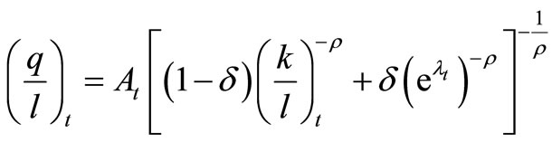
The model uses a CES-production function with a labour-augmenting factor, .
.
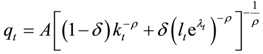 (1)
(1)
where  is investments in vehicles and
  employment in period t1.
The model also includes a Hicks neutral technical progress factor,  , where x is the expected increase in output capacity during the lifetime of the capital good and n is the planned length of life of the capital good.
2.1.2. Operating Costs
Over the length of life of an investment there arise operating costs in terms of wage costs and maintenance and repair costs. These costs are assumed to increase during the lifetime of the capital good.
The maintenance costs are assumed to be linked to the labour costs. The operating costs for a capital good of a specific age is then formulated 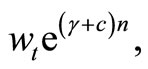 where
where  is the wage-rate at period t, γ is the expected wage increase during the lifetime of the capital good and c is a maintenance cost factor.
2.2. The Ex Ante Model
The entrepreneur calculates with a certain wage increase and a maintenance-cost during the investment’s length of life.
 (2)
(2)
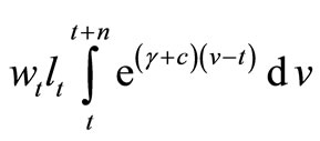
Production over time, in terms of value added, from the specific investment can be written
 (3)
(3)
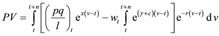
and the expected discounted profit of an investment is
 (4)
(4)
2.2.1. The Expected Length of Life
The production function is homogenous of degree one, which means that Equations (1) and (4), can be written in intensive form:
 (5)
(5)
and
 (6)
(6)
where PV is the present value per man hour of future surplus.
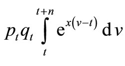
The discounted surplus of an investment in terms of net present value is,
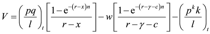 (7)
(7)
where  is the price of the investment good.
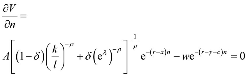
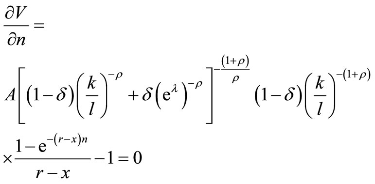
Dropping the time notation and assuming p = 1, differentiation of (7) gives:
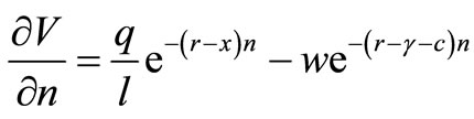 (8)
(8)
and the first-order condition becomes
 (9)
(9)
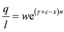
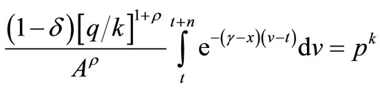
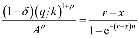
Figure 1 shows Equation (9), when γ, c, x > 0 and γ + c – x > 0.
The difference between  and
and  is the quasi-rent in each period generated by an investment and the discounted value equals the capital requirement per hour.
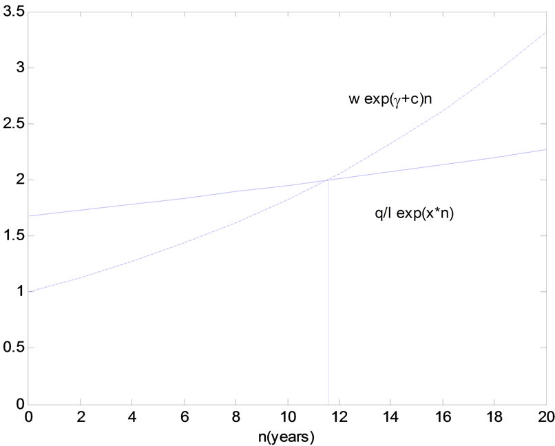
Figure 1. The ex ante length of life2. Baseline scenario: w = 1, r = 0.10, A = 1, δ = 0.6, ρ = 0.2, x = 0.015, γ = 0.02, c = 0.04, eλ = 1. Equilibrium values: q/l = 1.68, k/l = 4.15, n = 11.6.
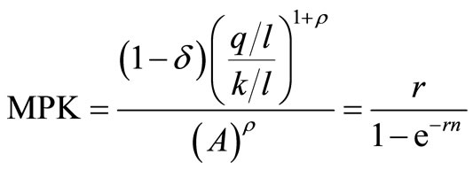
2.2.2. The Marginal Product of Capital
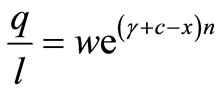
Maximizing the net present value (7) subject to the production function gives
 (10)
(10)
where  is the marginal product of capital (MPK).
Marginal productivity of capital for a new investment and the expected development of MPK over time are shown in Figure 2.
The firms invest in new capital until the discounted expected value of the marginal product of capital is equal to the price of the capital good ( = 1).
= 1).
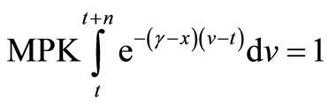 (11)
(11)
Equations (9) and (11) are necessary first order conditions for profit maximization. One interpretation of these conditions is that equation (11) concerns the intensive marginal, where the productivity of a new investment is determined, while equation (9), concerns the extensive marginal, where the ex ante length of life is fixed.
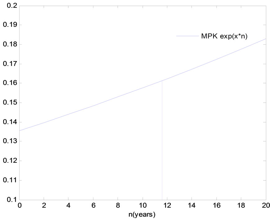
Figure 2. The marginal product of capital. Baseline scenario: w = 1, r = 0.10, A = 1, δ = 0.6, ρ = 0.2, x = 0.015, γ = 0.02, c = 0.04, eλ = 1. Equilibrium values: q/l = 1.68, k/l = 4.15, n = 11.6 and MPK = 0.1356.
3. Concavity and Comparative Statics
3.1. Concavity and Maximization
The first-order conditions (9) and (11) and the production function (5) give the following two equations:
 (12)
(12)
 (13)
(13)
The ex ante model, (12)-(13), contains two endogenous and two exogenous variables as well as seven parameters.
Endogenous variables: 
Exogenous variables: 

Parameters: 
The exogenous variables, w and r are determined by market forces. The parameters,  and
and , are determined by the existing technology, while
  and c are in accordance with the entrepreneur´s expectations of the future wage, productivity increase and maintenance and repair expenditure. Further, the labour-augmenting factor,
  is exogenously given.
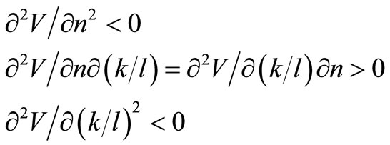
The profit function (7) is concave when
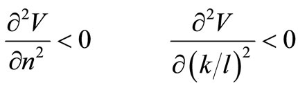
and
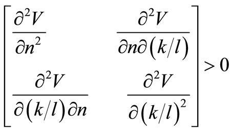
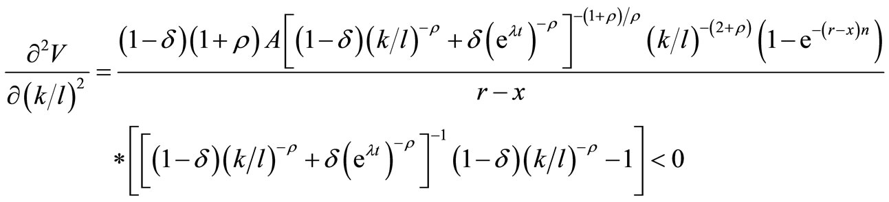
The second order partial derivatives are presented in Appendix A.
3.2. Comparative Statics
There is of some interest to study the effects of variations in the factor prices on the endogenous variables, n and .
.
Total differentiation of Equations (12) and (13) gives
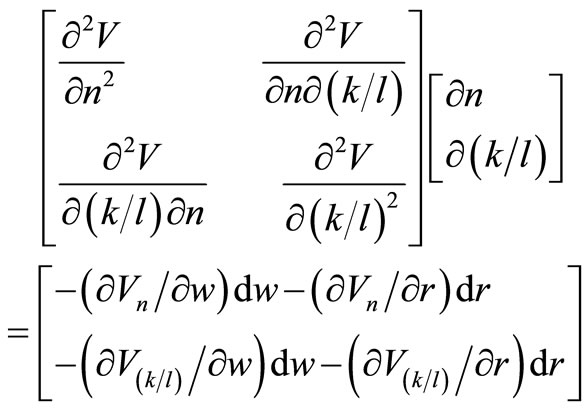 (14)
(14)
where
3.2.1. Variation in the Wage Rate, w
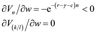
and
Using (14) and solving for 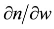 gives
gives
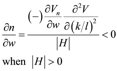
and
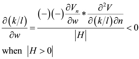
The implication of the model is that an increase in the wage rate will decrease the length of life of an investment and lower the capital intensity of the investment when the labour-augmenting factor is fixed, thus there is no technical progress. The first order condition (11) holds when the expected lifetime of the capital good decreases and the marginal product of capital increases in period t. The increase in the marginal product of capital implies that the factor intensity decreases due to diminishing returns to capital.
3.2.2. Variation in the Interest Rate, r

(14) gives
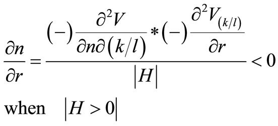
and
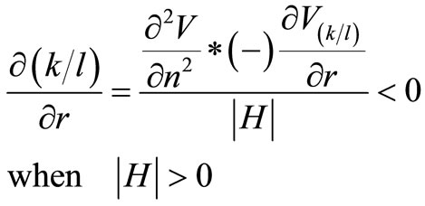
In this case an increase in the rate of interest will lower both the capital intensity of an investment and the lifetime of the capital good. The first-order condition (11) holds also in this case when the marginal product of capital increases in period t and the expected lifetime decreases.
3.3. Steady-State Properties of the Model
An economy displays steady-state properties when the capital-output ratio, the wage-share and other relevant variables remain constant over time. It can be shown that the derived model, that is, equations (5), (9) and (11)3 will follow a steady-state path when the wage rate changes at the same rate as the technical progress.
Equation (11) shows a constant output-capital ratio when the expected lifetime is constant.
 (11)
(11)
The link between the wage rate and the productivity is displayed by equation (9).
A fixed expected lifetime implies
Lastly, differentiation of the production function (5) gives
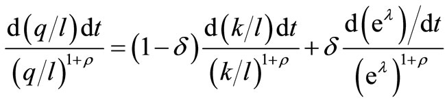 (15)
(15)
Equation (15) holds when
The derived model will, thus, generate equal growth paths for the productivity, capital intensity, labour augmenting factor ( ) and the wage-rate. This means that the wage-share,
  , and the output-capital ratio (
 ) for a new investment will remain constant.
3.4. Changes in the Wage Rate and Technical Progress
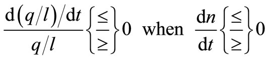
When the rate of technical progress equals the change in the wage rate, the model predicts a steady-state path of important variables. However, when the wages increase faster than the technical progress, the effects on n,  and
and  depend on the magnitude of technical progress and wage change, as well as the value of the substitution parameter.
There is now a possibility to use the two first-order conditions, (9) and (11), and the production function, (5), to derive an explicit relationship between the wage to technical progress ratio and the optimal lifetime of the capital good4.
Plug (9) and (11) into (5) and solve for 
 (16)
(16)
The graphical representation of equation (16) in Figure 3 reveals that there are two solutions.
The RHS of Equation (16) is increasing in n for lower values of n and decreasing for higher values. A given wage to technical progress ratio then implies that there are two solutions.5 However, concavity of the profit function (7) requires that the Hessian determinant is positive (see Section 3.1) and this condition holds when the RHS of (16) is decreasing in n. Thus, the profitmaximizing lifetime is to be found at the descending part of the curve.
A higher wage to technical progress ratio corresponds then to a lower optimal lifetime of a capital good. When there is no technical progress a higher wage gives the same outcome, which is in accordance with the result in Section 3.2.
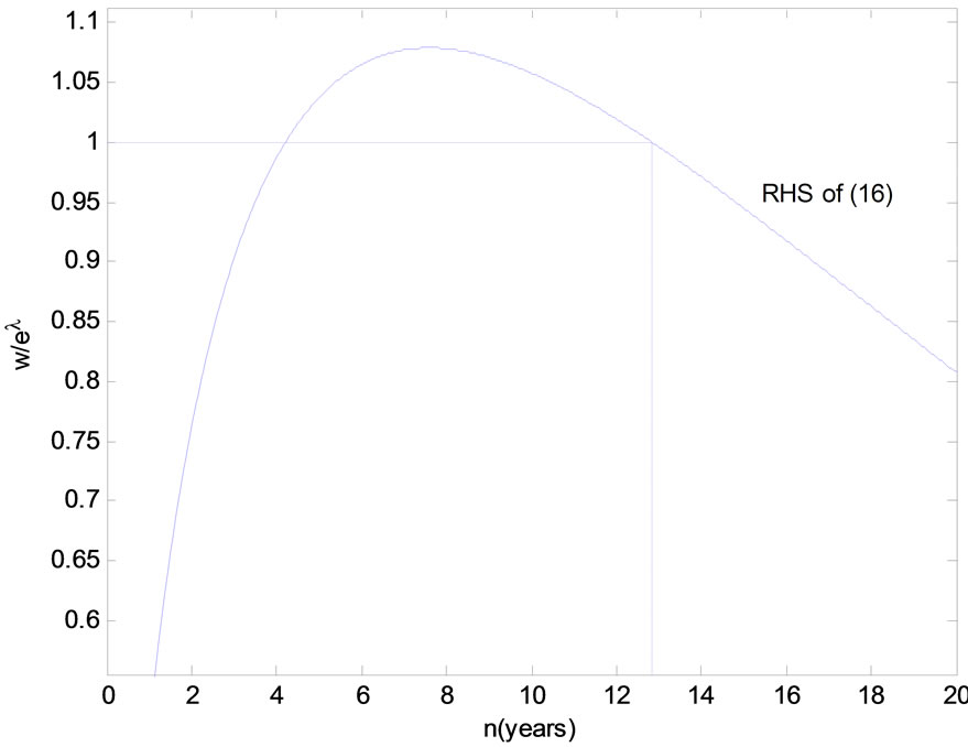
Figure 3. Expected lifetime of a capital good. Benchmark scenario: r = 0.10, A = 1, δ = 0.6, ρ = 0.2, c = 0.04, w = 1, eλ = 1, (w/eλ = 1). Benchmark equilibrium: q/l = 1.67, k/l = 4.05, n = 12.83.
The solution to equation (16) depends highly on the chosen values of the parameters in the model. The expected lifetime will be lower for a given wage to technical progress ratio when ,
,  , c and r become lower, while the lifetime increases when A rises.
However, when calibrating the model in order to mirror different real-world situations, for n,  and
and , there are usually minor problem arising.
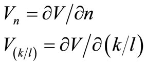
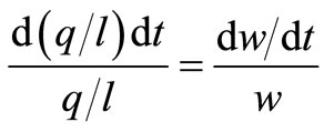
The productivity,  , of a new vintage is influenced by changes in the wage rate and the expected lifetime of the capital good. Assuming that
 , w and n are functions of t, differentiation of (9) gives:
 (17)
(17)
The absolute change in productivity depends on the magnitude of the wage change and the change in lifetime.
In order to eliminate different level effects when the substitution parameter changes, the parameters A and δ in the production function are calibrated to maintain the benchmark equilibrium for n,  and
and  in the system of equations (5), (9) and (11).
The effect on the lifetime of a change in the wage to technical progress ratio depends to a large extent on the value of the substitution parameter. The model predicts that a higher wage to technical progress ratio implies a lower lifetime6, but a higher  means that the change in the lifetime diminishes. Figure 4 shows the effect of a higher wage to technical progress ratio on the optimal lifetime at two different values of the substitution parameter.

Figure 4. Changes in wage to technical progress ratio (calibrated model). At A (benchmark equilibrium): w/eλ = 1, ρ = 0.2 or 0.4, n = 12.83; At B: w/eλ = 1.01, ρ = 0.2, n = 12.41; At C: w/eλ = 1.01, ρ = 0.4, n = 12.47.
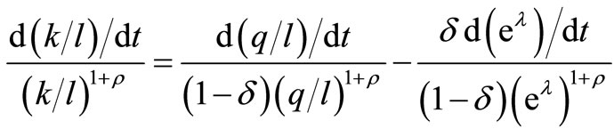
The effects on the capital intensity can be found by investigating equation (11) and the equation can be written:
 (18)
(18)
The RHS of (18) is decreasing in n, which means that a lower lifetime corresponds to a higher MPK.
Differentiating MPK = 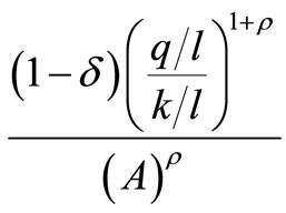 with respect to t gives
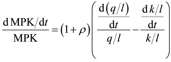 (19)
(19)
A higher MPK then implies
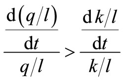 (20)
(20)
The inequality (20) implies that a positive change in  corresponds to either a negative or positive change in
 .
.
In order to indicate the effects on n,  and
and  when there is an increase in wage and technical progress, numerical solution of Equations (5), (9) and (11) will be performed.
Table 1 presents changes in n,  and
and  for a given change in the wage to technical progress ratio when the substitution parameter increases7.
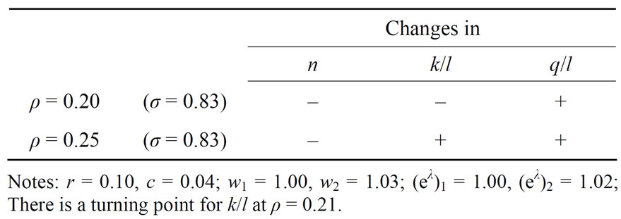
Table 1. Effects of a higher wage and technical progress ratio when deλ/dt > 0, (calibrated model).
A higher wage to technical progress ratio implies a lower expected lifetime of the investment and for a production function close to the Cobb-Douglas case the capital intensity will decrease while the factor productivity will increase. However, for firms with lower substitutability in production, the capital intensity as well as the factor productivity will increase.
The simulation results indicate that firms characterized by different elasticity of substitution will react differently with respect to the capital intensity when the wage to technical progress ratio changes.
3.5. Changes in the Interest Rate and Technical Progress
The RHS of (16) will shift downwards when the interest rate rises. The effects on the expected lifetime of a rise in the interest rate depend on the magnitude of technical progress as well as the value of the substitution parameter. When there is no technical progress a higher interest rate gives a lower lifetime and this result is shown in Figure 5. This specific outcome is in accordance with the result in Section 3.1.
The effects on MPK can be shown by investigating equation (18).

The RHS of (18) is decreasing in n and an increase in the interest rate will shift the curve upwards, which is shown in Figure 6.
A lower elasticity of substitution implies a lower substitutability in production. In order to compare the effects of a change in the interest rate at different values of ρ, the model is calibrated in the same way as in the previous section and the benchmark equilibrium is maintained for n,  ,
,  and MPK.
Figure 6 shows that a lower substitutability in production implies a lower change in MPK for a given change in the interest rate. Depending on the value of the substitution parameter, the expected lifetime will either decrease or increase when technical progress exists and the interest rate rises.
The change in the productivity can be found by investigation of equation (17) and  implies
The effect of an increased interest rate on the capital intensity will depend partly on the magnitude of the technical progress, partly on the value of the substitution parameter.
Equation (15) can be written
 (21)
(21)
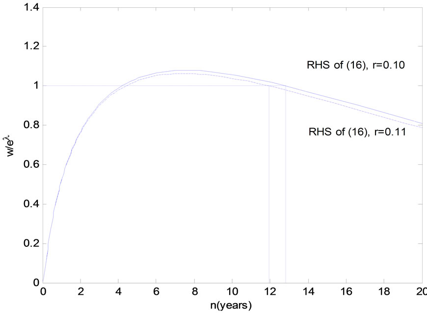
Figure 5. Increase in the interest rate. Benchmark scenario: w = 1, r = 0.10, A = 1, δ = 0.6, ρ = 0.2, c = 0.04, eλ = 1. Benchmark equilibrium: q/l = 1.67, k/l = 4.05, n = 12.8.
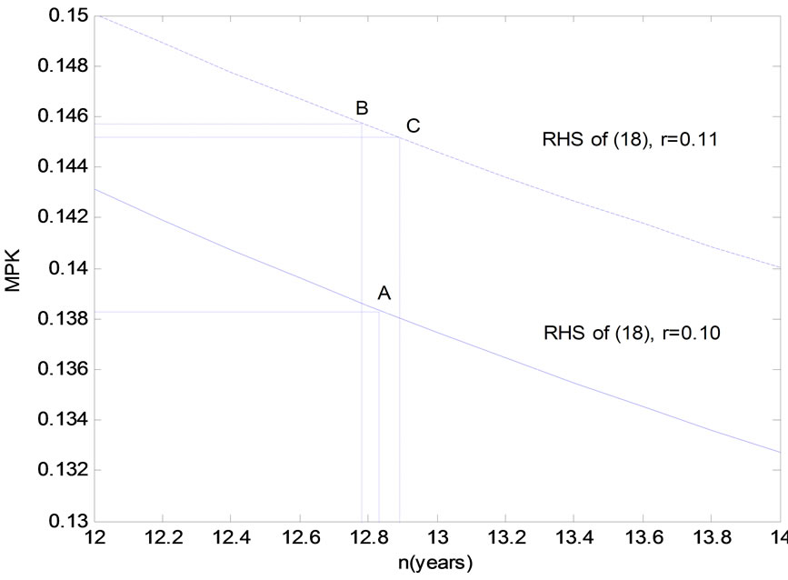
Figure 6. The effect on MPK and the expected lifetime of an increased interest rate when deλ/dt > 0 (calibrated model). At A (benchmark equilibrium: r = 0.10, eλ = 1, ρ = 0.2 or 0.4, MPK = 0.1383, n = 12.83; at B: r = 0.11, eλ = 1.02, ρ = 0.2, MPK = 0.1457, n = 12.78; at C: r = 0.11, eλ = 1.02, ρ = 0.4, MPK = 0.1452, n = 12.89.
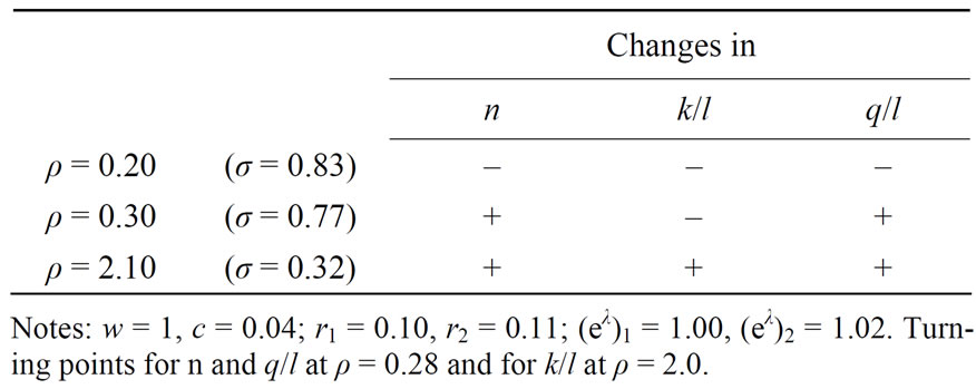
Table 2. Effects of a higher interest rate when deλ/dt > 0 (calibrated model).
A negative change in , means that
  will decrease when
 , while the change in
  is ambiguous when the productivity increases.
In order to show possible outcomes of an increased interest rate when the substitution parameter increases, numerical solutions of equations (5), (9) and (11) are presented in Table 2.
In the case with higher interest rate and , the effects on the three variables will change sign when the elasticity of substitution decreases.
4. Conclusions
The result of the presented investigation indicate that changes in the factor prices to a large extent influence the expected length of life and the factor intensity of a capital good. However, the effects depend highly on the value of the elasticity of substitution and the existence of technical progress.
An increased interest rate or wage rate will decrease the optimal lifetime of a capital good and the factor intensity when there is no technical progress.
Existence of technical progress means that the effect of a higher  on factor intensity depends on the elasticity of substitution. A function close to CobbDouglas production function implies that the factor intensity is decreasing in
 , while the reversed outcome arises at lower values of elasticity of substitution.
A higher interest rate and occurrence of technical progress means that different turning points exist for the optimal lifetime, factor intensity and factor productivity at different values for the elasticity of substitution. One important implication of these results is that an economic policy aiming at increasing investment in the economy, has to take into consideration that effects of changes in the factor prices to a large extent can depend on technical progress as well as the degree of substitutability in production.
5. Acknowledgements
I am grateful to Chuan-Zhong Li and Niklas Rudholm for valuable comments and important remarks on earlier versions. Seminar participants at Dalarna University have provided valuable comments on previous drafts of the manuscript. All remaining errors are my responsibility.
6. References
[1] L. Johansen, “Substitutions versus Fixed Production Coefficients in the Theory of Economic Growth: A Synthesis,” Econometrica, Vol. 27, No. 2, 1959, pp. 157-175. doi:10.2307/1909440
[2] W. E. G. Salter, “Productivity and Technical Change,” Cambridge University Press, Cambridge, 1960.
[3] R. M. Solow, “Substitution and Fixed Proportion in the Theory of Capital,” The Review of Economic Studies, Vol. 29, No. 3, 1962, pp. 207-218. doi:10.2307/2295955
[4] C. Bliss, “On Putty-Clay,” Review of Economic Studies, Vol. 35, No. 2, 1968, pp. 105-132. doi:10.2307/2296542
[5] L. Johansen, “Production Functions,” North-Holland, Amsterdam, 1972.
[6] E. Lundberg, ”Produktivitet och Räntabilitet,” SNS, Stockholm, 1961.
[7] K. J. Arrow, “The Economic Implications of Learning by Doing,” Review of Economic Studies, Vol. 29, No. 3, 1962, pp. 155-173. doi:10.2307/2295952
[8] H. Uzawa, ”Optimum Technical Change in an Aggregate Model of Economic Growth,” International Economic Review, Vol. 6, No. 1, 1965, pp. 18-31. doi:10.2307/2525621
[9] C. Burnside and M. Eichenbaum, “Factor-Hoarding and the Propagation of Business-Cycle Shocks,” The American Economic Review, Vol. 86, No. 5, 1996, pp. 1154-1174.
[10] J. M. Imbs, ”Technology, Growth and the Business Cycle,” Journal of Monetary Economics, Vol. 44, No. 1, 1999, pp. 65-80. doi:10.1016/S0304-3932(99)00013-6
[11] B.-H. Bahk and M. Gort, “Decomposing Learning by Doing in Plants,” Journal of Political Economy, Vol. 101, No. 4, 1993, pp. 561-583. doi:10.1086/261888
[12] R. Boucekkine, F. del Rio and B. Martinez, “Technological Progress, Obsolescence and Depreciation,” Oxford Economic Papers, Vol. 61, No. 3, 2006, pp. 440-466.
[13] C.-T. Hsieh, “Endogenous Growth and Obsolescence,” Journal of Development Economics, Vol. 66, No. 1, 2001, pp. 153-171. doi:10.1016/S0304-3878(01)00159-6
[14] G. Bitros, “The Optimal Lifetime an Assets under Uncertainty in the Rate of Embodied Technical Change,” Metroeconomica, Vol. 59, No. 2, 2008, pp. 173-188. doi:10.1111/j.1467-999X.2008.00298.x
[15] E. Bartelsman and M. Doms, “Understanding Productivity: Lessons from Longitudinal Microdata,” Journal of Economic Literature, Vol. 38, No. 3, 2000, pp. 569-595. doi:10.1257/jel.38.3.569
[16] J. M. Abowd, F. Kramarz and D. N. Margolis, “High Wage Workers and High Wage Firms,” Econometrica, Vol. 67, No. 2, 1999, pp. 251-333. doi:10.1111/1468-0262.00020
[17] J. Haltiwanger, J. Lane and J. Speltzer, “Productivity Differences across Employers: The Roles of Employer Size, Age, and Human Capital,” American Economic Review, Vol. 89, No. 2, 1999, pp. 94-98. doi:10.1257/aer.89.2.94
[18] M. Baily, E. Bartelsman and J. Halltiwanger, “Labor Productivity: Structural Change and Cyclical Dynamics,” Review of Economics and Statistics, Vol. 83, No. 3, 2001, pp. 420-433. doi:10.1162/00346530152480072
[19] K. Miyagiwa and C. Papageorgiou, “Elasticity of Substitution and Growth: Normalized CES in the Diamond Model,” Economic Theory, Vol. 21, No. 1, 2003, pp. 155-165. doi:10.1007/s00199-002-0268-9
[20] A. Dupuy and A. de Grip, “Elasticity of Substitution and Productivity, Capital and Skill Intensity Differences across Firms,” Economics Letters, Vol. 90, No. 3, 2006, pp. 340-347. doi:10.1016/j.econlet.2005.08.025
[21] O. de La Grandville, “In Quest of the Slutsky Diamond,” American Economic Review, Vol. 79, No. 3, 1989, pp. 468-481.
[22] R. Klump and O. de La Grandville, “Economic Growth and the Elasticity of Substitution: Two Theorems and Some Suggestions,” American Economic Review, Vol. 90, No. 1, 2000, pp. 282-291.
Appendix A:
Second-Order Partial Derivatives
 (A1)
(A1)
 (A2)
(A2)
 (A3)
(A3)
NOTES
1In the following sections and in the simulation parts the efficiency parameter, A, is assumed to be positive, while the distribution parameter, δ, can take values between 0 and 1. The model is investigated for production functions close to a Cobb-Douglas case, ρ→0, or closer to a fixed-proportions case, ρ→∞.
2Based on a numerical simulation of a system of equations, consisting of Equations (5), (9) and (11). The baseline scenario is characterized by a simple but still a fairly realistic description of some of the important variables in an economy in a specific period, t. In the baseline scenario the wage-share for a new investment approximately equals to 0.60 and the output-capital ratio roughly equals to 0.40. The labour-augmenting factor, λ, is exogenously given and eλ = 1 implies that λ = 0. Technical progress means that λt+1 > λt.
3Instead of investigating Equations (5), (9) and (11), Equations (12) and (13) could have been used.
4In Sections 3.4 and 3.5, x, γ = 0.
5Using different starting values in Matlab, numerical simulations of Equations (5), (9) and (11) will generate two solutions.
6At the descending part of the RHS of (16).
7The elasticity of substitution, σ = 1/(1 + ρ).
8((1 – () (k/l)–( + ( (e(t)–()(–1) (1 – () (k/l) –( < 1 when e(t > 0