Technology and Investment
Vol.2 No.2(2011), Article ID:5170,5 pages DOI:10.4236/ti.2011.22013
Are Trading Rules Profitable in Exchange-Traded Funds?
1Department of Economics and Hong Kong Institute of Asia-Pacific Studies,
The Chinese University of Hong Kong, Hong Kong, China
2Department of Economics, The Chinese University of Hong Kong, Hong Kong, China
E-mail: chong2064@cuhk.edu.hk
Received March 1, 2011; revised April 28, 2011; accepted May 4, 2011
Keywords: On-Balance Volume, Exchange-Traded Funds, Moving Average
Abstract
The Exchange-traded fund (ETF) is a burgeoning financial vehicle. Despite its growing importance, there has been a lack of empirical studies on the profitability of technical trading rules in the ETF market. This paper assesses the profitability of the On-Balance Volume indicator (OBV) on ETF trading. It is found that the trading rules associated with the OBV are able to generate handsome returns in the ETF market. This is in contrast to the conventional wisdom that funds should be bought and held.
1. Introduction
A wide variety of nascent financial vehicles have been developed in recent years. In particular, the Exchangetraded fund (ETF), among other financial innovations, has become a burgeoning financial vehicle and gained the attention of the populace. ETFs have a relatively short history. The world’s first ETF was launched in 1993, with a total asset value of US $484 million. By the end of 2010, there are over 1000 ETFs traded on US exchanges, with a total asset value of more than US $790 billion, reflecting a growing demand for this new financial vehicle.1 Compared to mutual funds, ETFs offer have a variety of advantages, such as a greater flexibility, lower fee, increased tax efficiency and greater transparency [1].2 Traditional performance metrics, such as Price/Earnings ratio and cash flow, cannot be applied to trade ETFs [2]. This paper examines a topical research area. Following Tsang and Chong [3], we evaluate the performance of the On-Balance Volume (OBV) indicator in the ETF market. The OBV is a simple indicator defined as:
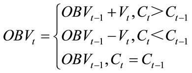
where Ct and Vt are the closing price and trading volume respectively at time t. We let OBV0 to be zero. A rising price together with a rising OBV indicates that the volume is heavier on up days, confirming the uptrend of the market. If prices are moving higher while the volume is falling, it suggests a trend reversal.
2. Data and Methodology
Our sample includes 30 US listed ETFs3 from six different categories, namely, Bear Market, Latin America, Telecommunications, Consumers Staples, Bond and Government Treasury Bills.4 Following Tsang and Chong [3], we employ the trading rules associated with the OBV indicator.5 Five trading rules are studied. The first four rules are based on the crossing of OBV and its n-day moving average, which is defined as:
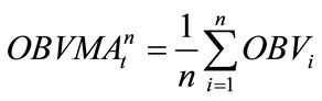
A trading signal is produced when OBV crosses the corresponding moving average. The fifth rule is based on the crossing of two OBV moving averages. The five OBV rules are defined as follows:
Rule 1: 10-day OBV
Buy at day t:  and
and 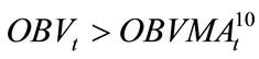
Sell at day t: 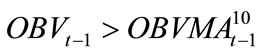 and
and 
Rule 2: 20-day OBV
Buy at day t:  and
and 
Sell at day t:  and
and 
Rule 3: 50-day OBV
Buy at day t:  and
and 
Sell at day t:  and
and 
Rule 4: 100-day OBV
Buy at day t: 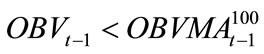 and
and 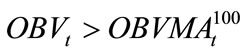
Sell at day t:  and
and 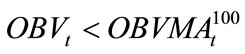
The fifth trading rule, which is based on the crossing of 10-day OBVMA and 20-day OBVMA, is defined as follows:
Rule 5: OBVMA10 × 20
Buy at day t: 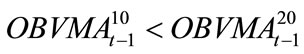 and
and 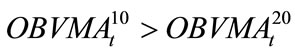
Sell at day t: 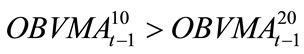 and
and 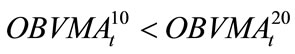
For the first four rules, a long position will be taken if OBV rises above the corresponding OBVMA, and liquidated when OBV falls below the corresponding OBVMA. The choices of the four window length n = 10, 20, 50 and 100 are common (Brock et al. [6], Tsang and Chong [3]). If a smaller value of n is used, there will be many noisy signals. For long-term investment, one may use a larger value of n to reduce the number of transactions.
We prohibit short-selling and consecutive buying/ selling in our calculation of returns.6 Transaction cost is assumed to be negligible. The performance of the five trading rules is evaluated in terms of the annualized rate of return. Since there are about 250 trading days each year, the annualized rate of return can be defined as follows:
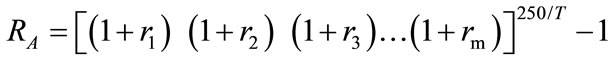
where
S(i) and B(i) are respectively the selling and buying prices of the ith transaction;
m is the number of transactions in the sample;
T is the number of trading days in the sample.7
To assess the impact of the 2008 Financial Tsunami on the profitability of our trading rules, we further split the whole sample into Pre-Tsunami and Post-Tsunami subsamples. The day when Lehman Brothers Holdings Inc. was delisted from the New York Stock Exchange, 17th September 2008, was set as the watershed. This is the major event that marks the onset of the Financial Tsunami. The daily closing prices and volume of each ETF are gleaned from DataStream. The details are reported in Table 1.
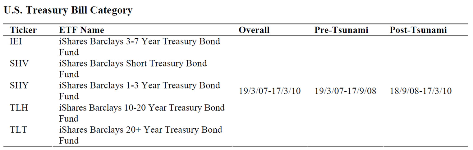
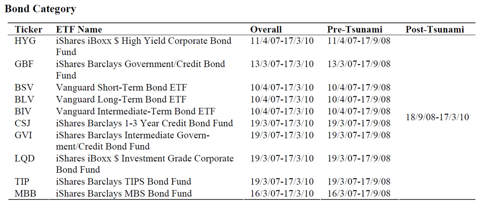
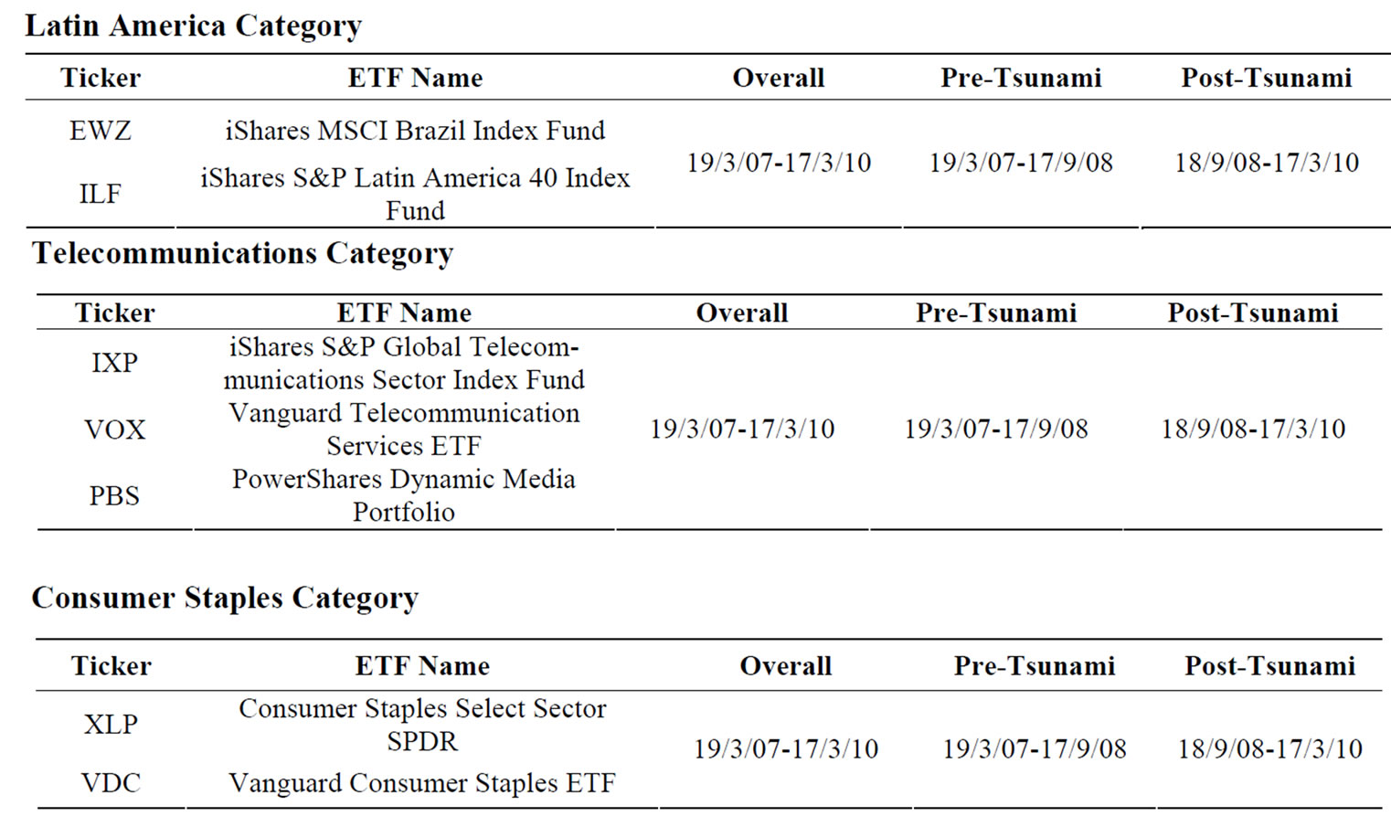
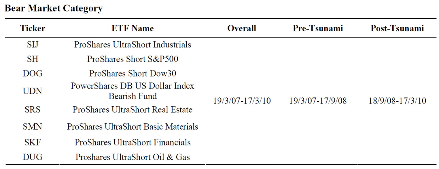
Table 1. ETF name list and time period.
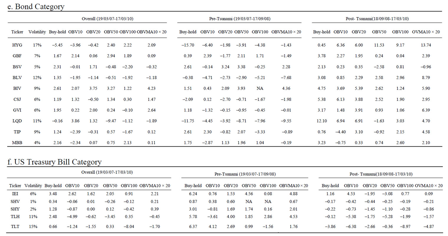
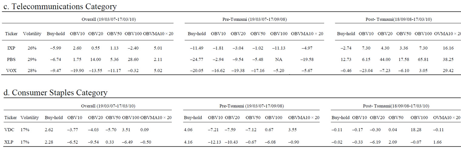
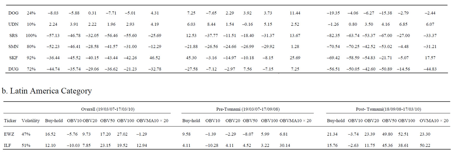
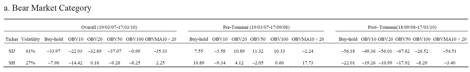
Table 2. a. Annual Rate of Return; b. Annual Rate of Return; c. Annual Rate of Return; d. Annual Rate of Return; e. Annual Rate of Return; f. Annual Rate of Return.
3. Results and Conclusions
Table 2 reports the annualized rate of return (in percentage) of our OBV trading rules. Note that the OBVMA10 × 20 rule performs consistently well in the three periods. For Bear Market and Latin America ETFs, the trading rules outstrip the buy-and-hold benchmark in almost all cases. Specifically, for the case of Proshares Ultrashort Financials (SKF), the OBVMA10 × 20 is able to achieve an annual rate of return of 47%. For the Bear Market ETFs, all the trading rules, especially OBVMA10 × 20, clearly dominate the buy-and-hold strategy. For ETFs in Bond, Telecommunications and Consumers Staples, our trading rules also beat the market in general. Note that the OBV trading rules excel in volatile markets. The higher the volatility, the better that the relative performance of the OBV rules. For ETFs associated with US Treasury Bills, the OBV trading rules fail to deliver a handsome return. For the whole sample period and pre-Tsunami period, the profits generated by the OBV trading rules are reasonably good. For the post-Tsunami period, our trading rules generate notably higher return than the benchmark. Overall, our results reveal that the OBV trading rule can beat the buy-and-hold strategy in the ETF market, especially for those ETFs with high volatility. This is in contrast to the conventional wisdom that funds should be bought and held.
4. References
[1] L. Carrel, “ETFs for the Long Run: What They Are, How They Work, and Simple Strategies for Successful LongTerm Investing,” Wiley, New York, 2008.
[2] D. Wagner, “Trading ETFs: Gaining an Edge with Technical Analysis (Bloomberg Market Essentials: Technical Analysis),” Bloomberg Press, New York, 2008.
[3] W. W. H. Tsang and T. T. L. Chong, “Profitability of the On-Balance Volume Indicator,” Economics Bulletin, Vol. 29, No. 3, 2009, pp. 2424-2431.
[4] J. H. Poterba and J. B. Shoven, “Exchange-Traded Funds: A New Investment Option for Taxable Investors,” American Economic Review, Vol. 92, No. 2, 2002, pp. 422-427. doi:10.1257/000282802320191732
[5] W. J. Trainor Jr., “Do Leveraged ETFs Increase Volatility,” Technology and Investment, Vol. 1, No. 3, 2010, pp. 215-220. doi:10.4236/ti.2010.13026
[6] W. Brock, J. Lakonishok and B. LeBaron, “Simple Technical Trading Rules and the Stochastic Properties of Stock Returns,” Journal of Finance, Vol. 47, No. 5, 1992, pp. 1731-1764. doi:10.2307/2328994
NOTES
1The exact number of ETFs depends on the definition employed, as there are many other ETF-like products listed in different exchanges [1].
2For recent studies on ETFs, see [4] and [5].
3According to the definition of Morning Star, ETFs that mainly hold US Treasury Bills are categorized as Short Government, Intermediate Government and Long Government. In our analysis, we define US Treasury Bills category as any ETFs falling into these three categories.
4These classifications, except for US Treasury Bills, are set by the ETFs’ corresponding issuers.
5We derive the OBV indicator using the trading volume of the ETFs, instead of the trading volume of the underlying assets.
6Short selling means the short selling of the ETF itself. ETFs in the Bear Market Category sometimes adopt a strategy of short-selling its underlying asset.
7Suppose we start with one dollar of investment, then [(1 + r1)(1 + r2)(1 + r3)…(1 + rm)] will be the total return after all the m transactions during period T. After taking the power of 250/T, and less the initial one dollar, we obtain the annualized rate of return.