Abstract

This paper demonstrates that continuation of traditional rate-of-return electric utility regulation of transmission and distribution assets will impede the ability of customers to optimize their generation portfolios. Under linear price regulation, with increasing (decreasing) returns to scale customers will choose a more (less) risky generation portfolio than they would with no transmission and distribution asset rate-of-return regulation. Similar problems arise under non-linear (two-part) pricing of transmission and distribution assets. When the per-unit price is set at marginal cost, with increasing (decreasing) marginal cost, customers will choose a more (less) risky generation portfolio than they would with no transmission and distribution asset regulation. With price caps the optimal generation portfolio is chosen.

1. Introduction

The US electric utility industry is currently in the middle of a massive transition from being a highly regulated industry to one that is partially deregulated. In the past, companies in the industry were vertically integrated with three distinct functional sectors: generation, transmission, and distribution. Those functions are being unbundled, either by regulatory fiat, or by the actual sell-off of assets. In the future, US consumers will have a rich array of choices with regard to generation sources, while the tranmission and distribution (T & D) sectors, and will still continue to be regulated by either state or federal commissions.¹

A major reason for this restructuring is to unleash competitive forces in the generation market, so as to decrease generation prices to the ultimate consumer. Consumers would also have a broader array of choices, in terms of price, price risk, and service quality. In particular, it is important that customers be allowed to optimize their portfolio in terms of generation price risk and price level without hindrance from regulators.

Unfortunately, because T & D assets are utilized to obtain the generation product, regulatory policies can have a bearing on customers’ decisions with regard to their generation portfolio mix. In particular, with traditional rateof-return regulation customers may choose a sub-optimal level of generation risk, a result that is inconsistent with the avowed desire to allow customers the opportunity to choose an optimal generation portfolio mix.² Consequently, the type of regulation currently employed in T & D regulation may have to be modified significantly.

In Section II we consider the market-induced trade-off between generation price risk and generation price level, and derive the unconstrained optimizing level of variance chosen by customers. This is used as a benchmark for Sections III and IV. In Section III we consider the impact of traditional rate-of-return regulation with linear pricing when T & D asset regulation is factored in. Section IV expands upon Section III by using non-linear regulatory pricing of T & D assets.

2. Unconstrained Model of Generation Portfolio Optimization

Assume a T & D utility that provides only regulated T & D services. Consumers purchase generation services in the competitive market on their own, with the electric energy transmitted over the T & D utility’s wires.

Define:

p = regulated price of T & D service;

E(.) = expectations operator;

u = stochastic disturbance term associated with the price of generation, where E(u) = 0;

s ² = E(u²) = variance in the price of generation;

g₀(s ²) + u = stochastic generation cost;

g₀(s ²) = E[g₀(s ²) + u] = expected generation cost;

q(p + g₀[s ²] + u ) = quantity demanded; and C(q) = cost function for providing T & D services.

Note that q is a function of the sum of T & D and generation prices.

Let the consumers’ utility function, for given u, be given as U(p + g₀[s ²] + u)). Assume this is of the Von Neuman-Morgenstern (V-M) type (see [5]). The utility function is, then, unique up to a linear transformation. In the selection of suppliers in the generation market by consumers, the expected generation price, g₀, obtainable by consumers is an inverse function of the variance, s ². In order to obtain a lower average generation price consumers have to accept a higher variance.³ This function can be reflected as g₀(s ²) where g' = ¶ g₀/¶ (s ²) < 0, and ¶ ²g₀ /¶ (s ²)² > 0.⁴

We can use a Taylor series approximation to express the expected utility of consumers as⁵

(1)

where U' = ¶U(p + g₀)/¶ p = ¶U(p + g₀)/¶ g₀ < 0. This represents the rate of change in utility with a change in generation price. Further, U" = ¶ ²U(p + g₀)/¶ p² = ¶ ²U(p + g₀)/¶ g₀². If consumers simply maximize their expected utility with respect to generation price variance, without any consideration of regulation on T & D operations, they would maximize (1) with respect to s ² producing

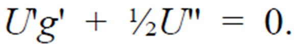(2)

This can be re-expressed as

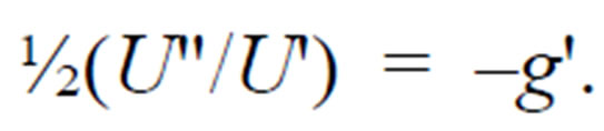. (3)

The Pratt-Arrow measure of absolute risk aversion with regard to price in this case is U"/U'.⁶ Equation (3) implies that utility maximization requires that one-half of the degree of absolute risk aversion be equal to the rate of trade-off between the level of generation prices and the variance of generation prices. If consumers are risk averse with regard to price, then U" < 0 and U"/U' > 0 because U' < 0. Since U is a V-M preference function, U"/U' is a unique measure (even with linear transformations). Let us assume constant absolute risk aversion so that U"/U' = j is constant, and is, consequently, independent of both the T & D price and the generation price.

As customers accept greater risk, s ², in their portfolio of generation sources, the expected generation price falls by an amount that is greater than the minimum required by customers. Without regulatory constraint, customers would optimally choose s₁² of generation portfolio variance. For variance less than s₁² an increase in s ² decreases g₀ by an amount greater than that amount required by consumers (given as ½j). For variance greater than s₁² a decrease in s ² increases g₀ by an amount less than that consumer would have been willing to bear.

3. Generation Portfolio Optimization with Regulation of T & D Assets Using Linear Pricing

Let us now explicitly introduce regulation of T & D assets into our model. Assume that g₀(s ²) + u and s ² are exogenously determined; that is, they are not determined by the regulator, but by competitive generation market conditions. We also assume that the regulated T & D utility has profit requirements on its T & D services, given as 0 ≤ E[pq – C(q)].⁷ This can be simplified to 0 ≤ pq₀ – C(q₀), where q₀ = q(p + g₀).⁸ In this case, the regulator's goal is to maximize E[U(p + g₀[s ²] + u])] with respect to p, subject to the profit constraint 0 = pq₀ – C(q₀). Customers maximize E[U(p + g₀[s ²] + u])] with respect to s ², subject to the same profit constraint.

The Lagrangian function is then

(4)

where l > 0 is the Lagrangian multiplier. Substitution from (1) into (4) yields the following Lagrangian expression

(5)

Assuming constant absolute risk aversion the firstorder conditions are:

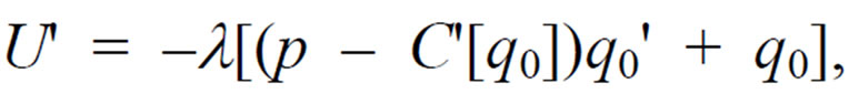(6)

(7)

where C' = ¶ C(q)/¶ q and q' = ¶ q/¶(p + g₀) = ¶ q/¶ p = ¶ q /¶ g₀.With increasing returns to scale, the term p – C'[q₀] is positive.⁹ Since l > 0, and g', q', U' < 0,

(8)

Consequently,

(9)

With the regulatory profit constraint on T & D assets, customers choose to have a generation portfolio variance of s₂² > s₁² which is a riskier generation portfolio than the portfolio they would choose without regulatory constraint on T & D assets (from in Section II).¹⁰

An intuitive explanation for this is that consumers have a regulatory-induced incentive to seek a greater amount of generation portfolio risk. That greater s₂² results in a lower value of g₀ and a corresponding greater amount of q. Given a regulatory constraint 0 < pq₀ - C(q₀), and since p – C'[q₀] > 0, consumers realize that with a larger s₂², the regulator will have to lower the regulated T & D price, p, with attendant T & D pricing benefits to the consumers. Consequently, by increasing s ² above s₁² consumers obtain the additional benefit of a correspondingly lower value of the T & D price, p.

Alternatively, with decreasing returns to scale, the term p – C'[q₀] is negative, and consumers choose s₃² < s₁² for their level of generation portfolio risk. That smaller s₃² results in a greater value of g₀ and a corresponding smaller amount of q. Given the regulatory constraint and since p – C'[q₀] < 0, consumers realize that with a smaller s₃² the regulator will have to lower the regulated T & D price, p, with attendant T & D pricing benefits to the consumers. Consequently, by decreasing s ² below s₁², consumers obtain a correspondingly lower value of the T & D price, p.

This sub-optimal behavior has effects on the size of the T & D system as well. Given the profit constraint pq₀ – C(q₀) = 0 we can calculate the change in p with a change in s ² by taking the total differential of the profit constraint:

(10)

which implies

(11)

The change in q₀ associated with a change in s ² is:

(12)

Substitution from Equation (11) into Equation (12) produces

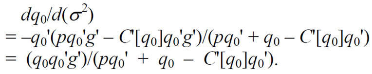(13)

The denominator of the above expression is the change in profits with a change in price, which is greater than zero by Equation (6). Further, since q₀', g' < 0, dq₀/d(s ²) > 0. As shown above, with increasing returns to scale, customers choose a riskier generation portfolio (s₂² > s₁² ). This implies that q₀, and the size of the T & D system is greater than it would be if customers had chosen the optimal generation portfolio variance, s₁². With increasing returns to scale, and rate-of-return regulation, the T & D system is larger than optimal.¹¹

The reason this sub-optimal behavior occurs is because of the responsiveness of q to g(s ²). We can evaluate that sensitivity by considering the impact of demand elasticity, e = –(¶ q₀/q₀)/(¶ p/p), on the amount by which s₂², or s₃², deviates from the optimal variance, s₁². Dividing (6) by (7) and rearranging terms produces

(14)

Dividing both sides of (14) by –q₀ and p produces:

(15)

where (p – C’)/p is the price mark-up (or mark-down). For a given price mark-up (or mark-down), the greater the elasticity, the greater the deviation of the consumers’ choice of sub-optimal variance from the optimal variance, s₁².

However, with price caps applied in regulation of T & D assets, customers no longer have an incentive to incur greater (or smaller) generation risk than is optimal.¹² A regulatory price cap, p_c, fixes prices for an indefinite period. As profits change, there are no offsetting changes in prices, as there is in traditional rate-of-return regulation. Consequently, consumers simply maximize

(16)

with respect to s ² to obtain the same result as in (3). Consumers will choose the optimal level of generation portfolio risk when price caps are applied to T & D regulation.

4. Generation Portfolio Optimization with Regulation of T & D Assets Using Non-Linear Pricing

Let us assume the same model as in Section III, but assume that the regulator employs non-linear pricing (two-part rates) with regard to the T & D assets.¹² Let the fixed T & D charge be F and the T & D per unit price be p. The consumers’ utility function is U(F, p + g₀[s ²] + u). Assume an income-compensated demand function of the form q(p + g₀[s ²] + u). Finally, assume that the regulator sets p equal to marginal cost, C', as is often the case in two-part pricing regimes.¹³ The regulatory profit constraint is 0 = E(F + [C'(q₀)q₀ – C(q₀)]), which can be simplified to 0 = F + [C'(q₀)q₀ – C(q₀)] [10-12]. In this case, the regulator's goal is to maximize E[U(F, p + g₀[s ²] + u)] with respect to F, subject to 0 = F + [C'(q₀)q₀ – C(q₀)]. Customers maximize E[U(F, p + g₀[s ²] + u)] with respect to s ², subject to the same profit constraint.

The Lagrangian is

(17)

with l > 0.The first-order conditions are:

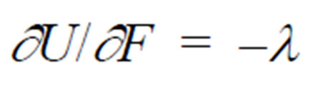(18)

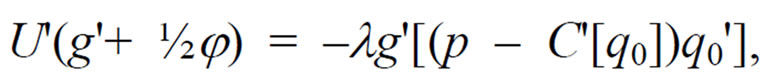
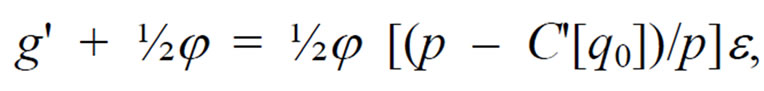
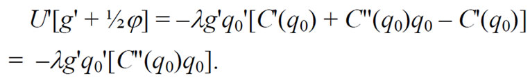(19)

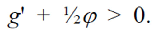
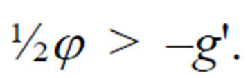
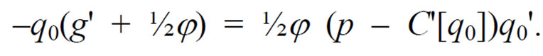
Increasing marginal cost, C"(q₀) > 0, implies that g' + ½j > 0 (since l > 0 and g', q', U' < 0). In that case consumers choose a level of variance that is greater than s₁², such as s₂². Conversely, decreasing marginal cost, C"(q₀) < 0, implies g' + ½j < 0. When that occurs, consumers choose a level of variance that is less than s₁², such as s₃². However, imposing price caps on the fixed charge and the per-unit price lead to the same optimal generation portfolio as in the linear pricing case.¹⁵

5. Conclusions

This paper has demonstrated that continuation of traditional rate-of-return electric utility regulation of transmission and distribution assets will impede the ability of customers to optimize their generation portfolios. Under linear price regulation, with increasing (decreasing) returns to scale customers will choose a more (less) risky generation portfolio than they would with no transmission and distribution asset rate-of-return regulation. Further, the size of the T & D system is greater (smaller) than optimal, with increasing (decreasing) returns to scale. The degree by which the portfolio variance deviates from the unregulated optimum increases as demand elasticity increases. However, with price cap regulation of transmission and distribution assets, consumers choose the optimal generation portfolio.

Similar problems arise under non-linear (two-part) pricing of transmission and distribution assets. When the perunit price is set at marginal cost, with increasing (decreasing) marginal cost, customers will choose a more (less) risky generation portfolio than they would with no transmission and distribution asset regulation. Setting a price cap on both the fixed charge and the per-unit price leads to the same optimal generation portfolio as in the linear pricing case.

This implies that the success of deregulation of electricity generation is closely intertwined with the type of regulatory regime employed by the regulator on those assets still under regulation. Rate-of-return regulation will cause sub-optimal results in the generation market. The regulator has to utilize alternative regulatory methods, such as price caps, so as to avoid unwanted interference in the generation market.

6. References

[1]       P. L. Joskow, “Restructuring, Competition and Regulatory Reform in the US Electricity Sector,” Journal of Economic Perspectives, Vol. 11, No. 3, Summer 1997, pp. 119-138.

[2]       S. Angle and G. Jr. Cannon, “Independent Transmission Companies: The For-Profit Alternative in Competitive Electric Markets,” Energy Law Journal, Vol. 19, No. 2, 1998, pp. 229-279.

[3]       J. C. Bonbright, A. L. Danielsen and D. R. Kamerschen, “Principles of Public Utility Rates,” 2nd Edition, Arlington, Public Utilities Reports, Inc., Virginia, 1980, pp. 573-575.

[4]       C. F. Jr. Phillips, “The Regulation of Public Utilities,” Arlington, Public Utilities Reports. Inc., Virginia, 1988.

[5]       I. Horowitz, “Decision Making and the Theory of the Firm,” Holt Rinehart and Winston, Inc., New York, 1970.

[6]       A. C. Chiang, “Fundamental Methods of Mathematical Economics,” 3rd Edition, McGraw-Hill, Inc., New York, 1984, pp. 257-258.

[7]       J. W. Pratt, “Risk Aversion in the Small and in the Large,” Econometrical, Vol. 32, No. 1-2, January-April 1964, pp. 122-136.

[8]       W. J. Baumol and D. F. Bradford, “Optimal Departures from Marginal Cost Pricing,” American Economic Review, Vol. 60, No. 3, 1970, pp. 265-283.

[9]       J. P. Acton and I. Vogelsang, “Introduction: Symposium on Price-cap Regulation,” Rand Journal of Economics, Vol. 20, No. 3, 1989, pp. 369-372.

[10]    T. R. Lewis and D. E. M. Sappington, “Regulating a Monopolist with Unknown Demand,” American Economic Review, Vol. 78, No. 5, December 1988, pp. 986-998.

[11]    K. E. Train, “Optimal Regulation: The Economic Theory of Natural Monopoly,” the MIT Press, Cambridge, Massachusetts, 1991.

NOTES

¹See [1] and [2] for an overview of electricity restructuring issues.

²See [3] and [4] for discussion of the rate-of-return method.

³Alternatively, we could say that in order to obtain lower price risk, market forces require the consumer to accept greater average generation prices.

⁴The positive sign of the second derivative implies that additional increments of risk reduce average generation price, in the market, by smaller and smaller amounts.

⁵A function f(x + a) can be expressed in a Taylor series as f(x) + a(( f/( x) + a²/2!(( ²f/( x²) + a³/3!(( ³f/( x ³) + …. [6]. A reasonable approximation is then f(x + a) = f(x) + a(( f/( x) + a²/2! (( ²f/( x²). Applied to this case, it implies that E[U(p + g₀[( ²] + u)] can be approximated as ( [U(p + g₀[( ²]) + uU'(p + g₀[( ²]) + ½u²U"( p + g₀[( ²])] du = U(p + g₀[( ²]) + E(u)U'(p + g₀[( ²]) + ½E(u²) U"( p + g₀[( ²]). Since E(u) = 0 and E(u²) = ( ², this produces U(p + g₀[( ²]) + E(u)U'(p + g₀[( ²]) + ½E(u²)U"(p + g₀[( ²]) = U(p+ g₀[( ²]) + ½( ² U"( p + g₀[( ²]).

⁶This can be seen from [7], Equations (4a)-(6), where we substitute p + g₀ for x.

⁷Throughout we assume that C(q) implicitly includes the cost of capital. See [8] for discussion of this point.

⁸Since q(p + g₀ + u) is stochastic, pq – C(q) is as well. Consequently, the constraint is expressed as 0 = E[pq – C(q)]. Using similar Taylor series expansion as discussed in footnote 5 we obtain E[pq – C(q)] = pq₀ – C(q₀) – ½( ²pq₀" – ½( ²C"(q₀)(q₀')² – ½( ² C'(q₀)q₀". The latter three terms are of small order of magnitude so that we can reasonably approximate E[pq – C(q)] as pq₀ – C(q₀).

⁹Since under rate-of-return regulation p = C/q, when C/q > C' we have increasing returns to scale.

¹⁰The average generation price is, also, lower than would be obtained without constraint. Our focus, however, in this paper is on generation portfolio variances.

¹¹With decreasing returns to scale, the T & D system would be smaller than optimal.

¹²See [2-4], and the “Symposium on Price-Cap Regulation” in [9] for discussion of price caps.

¹³See [10] and [11] for discussion of two-part tariffs.

¹⁴Similar to the discussion in footnote 8, 0 ≤ E(F + [C'(q₀)q₀ – C(q₀)]) can be approximated as 0 ≤ F + [C'(q₀)q₀ – C(q₀)] because of the relatively small order of magnitude of several terms in a Taylor series expansion.

¹⁵If a price cap is set on just the fixed charge or the per-unit charge, sub-optimal results are obtained.