Int'l J. of Communications, Network and System Sciences
Vol. 5 No. 3 (2012) , Article ID: 18001 , 5 pages DOI:10.4236/ijcns.2012.53023
The Injection Velocity and Apogee Simulation for Transfer Elliptical Satellite Orbits
Faculty of Information Technology, Polytechnic University of Tirana, Tirana, Albania
Email: Shkelzen.cakaj@fulbrightmail.org, {bkamo, vkolici, oshurdi}@fti.edu.al
Received December 27, 2011; revised January 26, 2012; accepted February 29, 2012
Keywords: Satellite; Orbit; Apogee; Perigee; Velocity
ABSTRACT
Basic resources for communication satellites are communication radio-frequencies and satellite orbits. An orbit is the trajectory followed by the satellite. The communication between the satellite and a ground station is established only when the satellite is consolidated in its own orbit and it is visible from the ground station. Different types of orbits are possible, each suitable for a specific application or mission. Most used orbits are circular, categorized as low, medium and geosynchronous (geostationary) orbits based on the attitude above the Earths surface. The launching process heading the satellite in geostationary orbit, by the first step places the satellite in a transfer orbit. The transfer orbit is elliptical in shape with low attitude at perigee, and the apogee of the geostationary orbit attitude. The apogee of the parking orbit depends on the injection velocity applied at perigee. Simulation approach of injection velocity at perigee to attain different apogees, considering an incremental step is presented in this paper.
1. Introduction
The satellite systems dedicated for global coverage are comprised of constellations of low Earth orbit (LEO) and geostationary Earth orbit (GEO) satellites [1]. The satellite’s launching process toward geostationary orbit because of too large distance form the Earth, takes few steps. In the first step the satellite is injected into a low Earth circular orbit (LEO). In the second step, the satellite’s orbit is transformed from the low Earth orbit into an elliptical transfer orbit by maneuvers at perigee, in order to attain the apogee equal to geostationary (GEO) orbit’s radius. Finally, the satellite is placed from the elliptical transfer orbit to the final destination, as geostationary orbit [2,3]. The geostationary orbit is unique faced with too close proximity of satellites in this orbit. To avoid mutual interferences and collision, a method of multi-satellites separation has to be applied [4].
This paper is concerned about the second phase of launching process; concretely the simulation of the transformation process from a low Earth orbit to an elliptical transfer orbit considering different low Earth orbit attitudes is given. Through analysis and simulation it is calculated what injection velocity has to be applied at low Earth orbit in order to attain the apogee which corresponds to the radius of final planned orbit.
Firstly, the parameters of elliptical orbit are given, then the relationship between the injection velocity at perigee and apogee incremental step is concluded. This mathematical relationship is further applied for simulation model, and finally simulation results are provided.
2. Elliptical Orbits
The path of the satellite’s motion is an orbit. Generally, the orbits of communication satellites are ellipses laid on the orbital plane defined by space orbital parameters. These parameters (Kepler elements) determine the position of the orbital plane in space, the location of the orbit within orbital plane and finally the position of the satellite in the appropriate orbit [5-7]. The exactly know position of the satellite in space enables the communication between the satellite and ground stations (users) [8].
The communication between the satellite and a ground station is established only when the satellite is stabilized in its own orbit. Thus, permanent attitude control is mandatory. In terms of attitude control performance the satellite reaction wheel’s configuration plays also an important role in providing the attitude control torques [9]. Different algorithms are applied and active control means are generally added to assure accurate attitude stabilization, keeping the attitude errors within permitted limits, consequently keeping the quality of communication [10, 11].
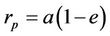
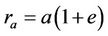
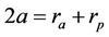
The elliptical orbit is determined by the semi-major axis which defines the size of an orbit, and the eccentricity which defines the orbit’s shape. Orbits with no eccentricity are known as circular orbits. The elliptical orbit shaped as an ellipse, with a maximum extension from the Earth center at the apogee (ra) and the minimum at the perigee (rp) is presented in Figure 1.
Figure 2 provides different orbits related to the Earth. Three of them are circular orbits (geosynchronous and medium) and the forth one is the well known Russian Molniya elliptical orbit. Too low perigee and too high apogee of elliptical orbit are obvious at Figure 2. The large difference between apogee and perigee causes high eccentricity.
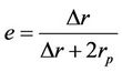
The orbit’s eccentricity is defined as the ratio of difference to sum of apogee (ra) and perigee (rp) radii as Equation (1) [5-7].
 (1)
(1)
Applying geometrical features of ellipse yield out the relations between semi major axis, apogee and perigee:
 (2)
(2)
 (3)
(3)
 (4)
(4)
both, rp and ra are considered from the Earth’s center. Earth’s radius is  km. Then, the attitudes (highs) of perigee and apogee are:
 (5)
(5)
 (6)
(6)
3. Injection Velocity and Orbits
Different methods are applied for satellite injection missions. Goal of these methods is to manage and control the satellite to safely reach the low Earth orbit, and then transfer elliptical orbit and finally geostationary orbit [12- 14].
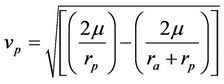
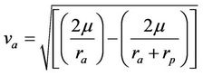
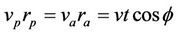
The specific orbit implementation depends on satellite’s injection velocity. The orbit implementation process on the best way is described in terms of the cosmic velocities. Based on Kepler’s laws, considering an elliptical orbit, the satellite’s velocity at the perigee and apogee point, respectively are expressed as [2]:
 (7)
(7)
 (8)
(8)
 (9)
(9)
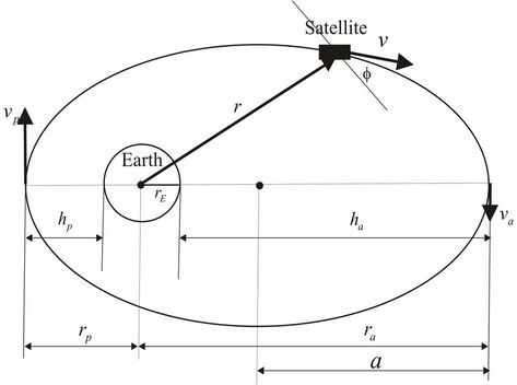
Figure 1. Major parameters of an elliptical orbit.
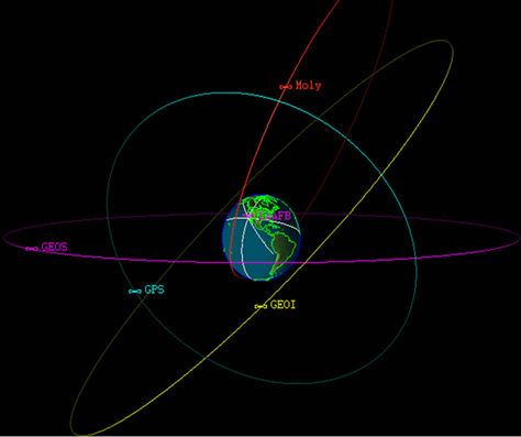
Figure 2. Satellite orbits.
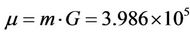 km3/s2. G is the Earth’s gravitational constant and m is Earth’s mass.
  represents an angle between a satellite vector r and local horizon at satellite point. For orbit with no eccentricity (e = 0), apogee and perigee distances are equal (ra = rp = a), thus orbit becomes circular with radius a and orbital velocity as [2]:
 (10)
(10)
By definition this is called the first cosmic velocity, enabling the satellite to orbit circularly around the Earth at uniform velocity according to Equation (10). If the injection velocity happens to be less than the first cosmic velocity, the satellite follows a ballistic trajectory and falls back to Earth [2]. The second cosmic velocity is defined as:
 (11)
(11)
Under the second cosmic velocity at perigee, the apogee distance ra infinitely increases, so the satellite escapes Earth’s gravitational pull. The trajectory is a parabola and eccentricity is equal to 1. For injection velocity rp at perigee more than the first cosmic velocity and less than the second cosmic velocity, the orbit is elliptical with an eccentricity in between 0 and 1. This is expressed as:
 (12)
(12)
 (13)
(13)
The satellite injection point is at perigee, and the apogee distance attained in the elliptical orbit depends upon the injection velocity. The higher the injection velocity at perigee, the greater is the apogee distance, as schematically is presented in Figure 3. For the same perigee distance rp, if under the injection velocity vp1 at perigee it is attained an apogee distance ra1, and under velocity vp2 it is attained an apogee distance ra2, then applying Equation (7) yields the relationship between velocities at perigee and respective attained distances at apogee (Equation (14)).
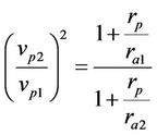 (14)
(14)
By definition, the apogee distance is always larger than the perigee distance, thus it can be expressed as:
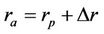 (15)
(15)
where  represent the distance of how much it is intended to achieve larger apogee compared with perigee of the orbit. This is defined as apogee incremental step. Applying Equation (15) at Equations (1) and (7) yield out Equations (16) and (17).
 (16)
(16)
 (17)
(17)
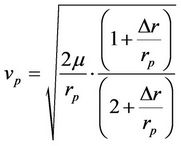
Equation (16) expresses how the eccentricity changes with , respectively how the eccentricity changes with the apogee incremental step keeping the fixed perigee. The Equation (17) tells us, which injection velocity rp has to be applied at perigee point in order to attain apogee for
  larger than in advance defined perigee. For
 , the orbit is circular, (e = 0) and according to Equation (17) orbital velocity is the first cosmic velocity.
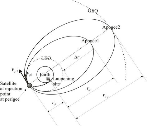
Figure 3. Injection velocity and attained apogee.
4. The Simulation and Results
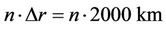
For the simulation purposes it is considered fixed perigee. Four fixed perigee distances are considered as: 7000 km, 7200 km, 7400 km and 7600 km. Considering Equation (5), and Earth’s radius  km, these perigee distances correspond to highs above Earths surface (attitudes) approximately of 600 km, 800 km, 1000 km and 1200 km, which are usually the attitudes of low Earth orbits at the first step of launching process. The apogee increase is considered by n steps, as:
 (18)
(18)
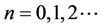 . For n = 0, the orbit is circular with low attitude, and for n = 19 the apogee distance achieves approximately the radius of geostationary orbit. In between these two cases fall medium attitudes for medium orbit satellites. Based on this approach firstly it is analyzed the eccentricity variation because of apogee increment, presented in Figure 4 and confirming eccentricity increment with apogee increase. It is too low eccentricity’s variation for different perigees, since the considered perigees are too close to each other. Finally, the goal of the paper is to conclude about the required velocity at injection perigee point as a function of the apogee increment. For this purpose it is applied Equation (17), and results are presented in Table 1 and Figure 5.
Figure 5 shows four curves for different perigee values, respectively corresponding to low Earth orbit attitudes of 600 km, 800 km, 1000 km and 1200 km. For attitude of 600 km (perigee of 7000 km) the injection velocity at perigee point is 7.55 km/s and for attitude of 1200 km (perigee of 7600 km) the injection velocity at perigee is 7.24 km/s. As higher perigee (higher attitude) the lower injection velocity is required at perigee point. Obviously, for defined low Earth orbit the higher velocity
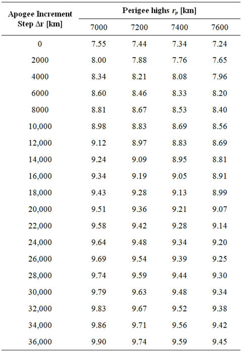
Table 1. Injection velocity [km/s].
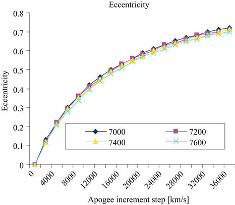
Figure 4. Eccentricity variation.
is required at perigee in order to attain larger apogee. For an in advance determined apogee, from Figure 5 can be found out what is required velocity at perigee point to attain respective apogee.
Let us consider this relation from the point of view of different low Earth orbit attitudes. For example, in order
Figure 5. Injection velocity and attained apogee.
to attain an apogee of 42400 km (corresponds to geostationary attitude) from the low earth orbit with a perigee of 7400 km (low earth attitude of 1000 km) the applied velocity at perigee must be 9.59 km/s. In order to attain the same apogee from the higher low earth orbit of attitude of 1200 km (perigee of 7600 km) the lower velocity is required to be applied at perigee point, concretely as 9.45 km/s. This means, in order to attain the geostationary attitude less velocity has to be applied at higher low Earth orbit attitude.
5. Conclusion
The satellite’s launching process toward geostationary orbit takes few steps. The first one positions the satellite at low Earth orbit. At the second step of this process the satellite is positioned at highly elliptical transfer orbit. For the fixed perigee of the elliptical transfer orbit, the attained apogee depends on injection velocity at perigee point. The greater injection velocity from the first cosmic velocity, the greater is the apogee distance attained. Curves provided can be applied to find out the attained apogee high for a given value of injection velocity at the perigee point, or on the other hand for required apogee what injection velocity has to be applied. It is confirmed, that in order to attain apogees of (7000 - 42,400) km the injection velocity to be applied at perigee point ranges at (7.24 - 9.90) km/s. The transformation process from transfer elliptical orbit to the final orbit, it is not treated within this paper.
REFERENCES
- O. Hoernig and D. Sood, “Military Applications of Commercial Communications Satellites,” Military Communications Conference Proceedings, Atlantic City, 31 October-3 November 1999, pp. 107-111.
- A. Maini and V. Agrawal, “Satellite Technology,” Wiley, London, 2010. doi:10.1002/9780470711736
- E. C. Lorenzini, et al., “Mission Analysis of Spinning Systems for Transfers from Low Orbits to Geostationary,” Journal of Spacecraft and Rockets, Vol. 37, No. 2, 2000, pp. 165-172. doi:10.2514/2.3562
- L. Jiancheng, “Separation of Geostationary Satellites with Eccentricity and Inclination Vector,” Proceedings: International Conferece on Measuring Technology and Mechatronics Automation, Changsha, 11-12 April 2009, pp. 855-858.
- D. Roddy, “Satellite Communications,” McGraw Hill, New York, 2006.
- M. Richharia, “Satellite Communication Systems,” McGraw Hill, New York, 1999.
- Sh. Cakaj, “Intermodulation Interference Modelling for Low Earth Orbiting Satellite Ground Stations,” Modelling, Simulation and Optimization, I-Tech, Vienna, 2009, pp. 1-20.
- Sh. Cakaj, “Horizon Plane and Communication Duration for Low Earth Orbiting (LEO) Satellite Ground Stations,” Transactions on Communications, Vol. 8, No. 4, 2009, pp. 373-383.
- Z. Ismail and R. Varatharajoo, “A Study of Reaction Wheel Configuration for a 3-Axis Satellite Attitude Control,” Advances in Space Research, Vol. 45, No. 6, 2009, pp. 750-759. doi:10.1016/j.asr.2009.11.004
- R. Esmailzadeh, H. Arefkhani and S. Davoodi, “Active Control and Attitude Stabilization of a Momentum-Biased Satellite without Yaw Measurements,” Proceedings of 19th Iranian Conference on Electrical Engineering, Tehran, 17-19 May 2011, pp. 1-6.
- M. Reyhanoglu and S. Drakunov, “Attitude Stabilization of Small Satellites Using Only Magnetic Actuation,” 34th Conference on Industrial Electronics, Orlando, 10-13 November 2008, pp. 103-107. doi:10.1109/IECON.2008.4757936
- H. Min, et al., “Optimal Collision Avoidance Maneuver Control for Formation Flying Satellites Using Linear Programming,” Proceedings of 29th Chinese Control Conference, Beijing, 29-31 July 2010, pp. 3390-3393.
- A. Mohammadi, et al., “On Application of Q-Guidance Method for Satellite Launch Systems,” 3rd International Symposium on Systems and Control in Aeronautics and Astronautics, Harbin, 8-10 June 2010, pp. 1314-1319. doi:10.1109/ISSCAA.2010.5632295
- J. Pearson, “Low Cost Launch Systems and Orbital Fuel Depot,” Acta Astronautica, Vol. 18, No. 4, 1999, pp. 315-320.