Int'l J. of Communications, Network and System Sciences
Vol.4 No.2(2011), Article ID:4026,11 pages DOI:10.4236/ijcns.2011.42014
A Novel Symbolic Algorithm for Maximum Weighted Matching in Bipartite Graphs*
School of Computer Science and Technology, Guilin University of Electronic Technology, Guilin, China
E-mail: gu@guet.edu.cn
Received December 2, 2010; revised January 17, 2011; accepted January 20, 2011
Keywords: Bipartite Graphs, Weighted Matching, Symbolic Algorithm, Algebraic Decision Diagram (ADD), Ordered Binary Decision Diagram (OBDD)
Abstract
The maximum weighted matching problem in bipartite graphs is one of the classic combinatorial optimization problems, and arises in many different applications. Ordered binary decision diagram (OBDD) or algebraic decision diagram (ADD) or variants thereof provides canonical forms to represent and manipulate Boolean functions and pseudo-Boolean functions efficiently. ADD and OBDD-based symbolic algorithms give improved results for large-scale combinatorial optimization problems by searching nodes and edges implicitly. We present novel symbolic ADD formulation and algorithm for maximum weighted matching in bipartite graphs. The symbolic algorithm implements the Hungarian algorithm in the context of ADD and OBDD formulation and manipulations. It begins by setting feasible labelings of nodes and then iterates through a sequence of phases. Each phase is divided into two stages. The first stage is building equality bipartite graphs, and the second one is finding maximum cardinality matching in equality bipartite graph. The second stage iterates through the following steps: greedily searching initial matching, building layered network, backward traversing node-disjoint augmenting paths, updating cardinality matching and building residual network. The symbolic algorithm does not require explicit enumeration of the nodes and edges, and therefore can handle many complex executions in each step. Simulation experiments indicate that symbolic algorithm is competitive with traditional algorithms.
1. Introduction
The matching problems find their applications in many settings where we often wish to find the proper way to pair objects or people together to achieve some desired goal. The matching problems are classified into maximum cardinality matching in bipartite graphs, maximum cardinality matching in general graphs, maximum weighted matching in bipartite graphs, and maximum weighted matching in general graphs [1,2]. The first is looking for a matching with the maximum edges, in which nodes are partitioned into boys and girls, and an edge can only join a boy and a girl; The second is the asexual case, where an edge joins two persons; In the third, we still have nodes representing boys and girls, but each edge has a weight associated with it. Our goal is to find a matching with the maximum total weight. This is the well-known assignment problem of assigning people to jobs and maximizing the profit; The fourth is obtained from the first one by making it harder in both ways.
Formally, a bipartite graph is a graph  in which
 ,
,  ,
,  and
and . A matching in G is a subset of edges,
  , such that each node in
  is an endpoint of at most one edge in M. The cardinality
  of a matching M is the number of edges in M. A matching which contains a maximum number of edges is called the maximum-cardinality matching. A weighted bipartite graph is a graph
 , where
  (non-negative real number) is a weight function, by which each edge
  is associated with a weight
 . The weight of a matching M is the sum of the weights of edges in the matching, i.e.,
 . Maximum weighted matching problem in bipartite graphs is finding a matching with the maximum weight or a maximum-cardinality matching with the maximum weight. In this paper, we consider the latter case. The classical Hungarian method was invented by Kuhn [3], which solves maximum weighted matching problems in strongly polynomial time of
 . It was revised by Munkres, and has been known since as the Hungarian algorithm or the Kuhn-Munkres algorithm (KMA) [1,4]. Under the assumption of integer weights in the range
 , Gabow and Tarjan used cost scaling and blocking flow techniques to obtain an
  time algorithm [5]. Algorithms with the same running time bound based on the push-relabel method were developed by Goldberg, Plotkin, Vaidya, Orlin and Ahuja [6,7]. Goldberg and Kennedy implemented the scaling push-relabel method in the context of assignment problems, known as cost scaling algorithm (CSA) [8], which is very competitive for practical use.
Finding maximum weighted matching in bipartite graphs is one of typical combinatorial optimization problems, where the size of graphs is a significant and often prohibitive difficulty. This phenomenon is known as combinatorial state explosion, resulting in that large graphs cannot be stored and operated on even the largest contemporary computers. In recent years, implicitly symbolic representation and manipulation technique, called as symbolic graph algorithm or symbolic algorithm [9,10], has emerged in order to combat or ease combinatorial state explosion. Typically, ordered binary decision diagram (OBDD) or algebraic decision diagram (ADD) or variants thereof are used to represent the discrete objects. Efficient symbolic algorithms have been devised for hardware verification, model checking, testing and optimization of circuits [9-13]. Hachtel and Somenzi developed OBDD-based symbolic algorithm for maximum flow in 0-1 networks that can be applied to very large graphs (more than 1036 edges) [14]. Bahar et al. present Algebraic Decision Diagram (ADD) to support algebraic and arithmetic operations on the general objects, and develop the symbolic algorithms for matrix multiplication, all-pair shortest path and timing analysis of combinational circuits [15]. Gu and Xu presented the symbolic ADD (Algebraic Decision Diagram) formulation and algorithms for maximum flow problems in general networks [16]. Symbolic algorithms appear to be a promising way to improve the computation of large-scale combinatorial optimization problems through encoding and searching nodes and edges implicitly. Our contribution is to present the symbolic algorithm for maximum weighted matching in bipartite graphs.
The rest of this paper is organized as follows. In Section 2, we introduce some backgrounds regarding maximum weighted matching in weighted bipartite graphs; Section 3 presents the symbolic formulations for weighted bipartite graphs and maximum weighted matching problems; In Section 4, we give the symbolic formulations for weighted bipartite graphs and maximum weighted matching problems; Section 5 presents the symbolic ADD algorithm; In Section 6, some experimental results and analysis are provided; The last section gives some conclusions.
2. Backgrounds
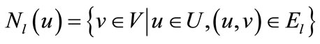
A bipartite graph  is a graph whose node set can be partitioned into two non-empty disjoint groups U and V such that every edge of the graph is incident on at most one node from each group. A matching M of G is a subset of edge set E such that no two elements of M are incident to the same node. A perfect matching is a matching M in which every node is adjacent to some edge in M. We refer to the edges in M as matched edge, and edges not in M as unmatched or free edges. We also refer to a node w as matched node with respect to a matching M if there is an edge in M incident to node w, and it is called free or unmatched otherwise. For a matched node u the unique node v connected to u by a matching edge is called the mate of u. The cardinality
  of a matching M is the number of edges in M. A matching which contains a maximum number of edges is called a maximum-cardinality matching.
A simple path p in G is called an alternating path with respect to the matching M if the edges in p are alternately in M and not in M. We refer to an alternating path as an even alternating path if it contains an even number of edges and an odd alternating path if it contains an odd number of edges. An odd alternating path with respect to a matching M is called as an augmenting path if the first node and last node in the path p are unmatched or free.
This particular structure of bipartite graphs can be used in developing the algorithms. We can direct all unmatched edges from U to V and all matched edges from V to U, and refer to the directed bipartite graph  as a residual network with respect to bipartite graph G and matching M. On the directed view, the existence of an augmenting path is then tantamount to the existence of a path from a free node in U to a free node in V. Also, augmenting by a path p is trivial. One simply reverses the direction of all edges on the path. Observe that this correctly records that the endpoints of p are now matched and that M is replaced by
 .
.
Property 1 If p is an augmenting path with respect to a matching M, then 
 is also a matching of cardinality |M| + 1. Moreover, in the matching
 , all the matched nodes in M remain matched, and two additional nodes, namely the first and last nodes of p, are matched.
Property 2 If  holds for two matchings M1 and M2 of G, then there are
  augmenting paths with respect to M1 in G, and the paths are node-disjoint.
Property 2 guarantees the existence of many augmenting paths when current matching is still far from optimality, and suggests organizing many node-disjoint augmenting paths in each execution. In this regard, layered networks are usually constructed. In a layered network the nodes of a graph are partitioned into layers according to their distance with respect to the starting layer, i.e., a node w belongs to layer k if there is a path from the starting layer to w consisting of k edges and there is no path with fewer edges. For any edge in a layered network the distance of the target node is at most one more than the distance of the source node. The construction of the layered network begins by putting all free nodes in U into the zeroth layer, and then proceeds by breadth-first search. The first layer is completed that contains free nodes in V, and the second layer contains free nodes in U and so on. Only edges that connect different layers can be contained in shortest augmenting paths, and the layered network contains all augmenting paths of shortest length.
A weighted bipartite graph is a graph , where
  (non-negative real number) is a weight function, by which each edge
  is associated with a weight
 . The weight of a matching M is the sum of the weights of edges in the matching, i.e.,
 . A maximum weighted matching is a perfect matching with the maximum weight.
In a weighted bipartite graph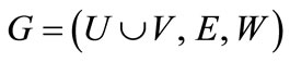 , a node labeling is defined by the labeling function
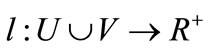 , and a feasible labeling is one such that
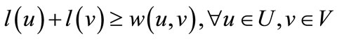 (1)
(1)
With respect to a feasible labeling l, the equality bipartite graph is referred as
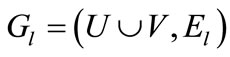 (2)
(2)
where
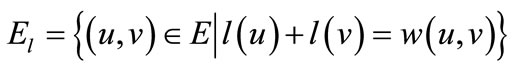 (3)
(3)
Property 3 (Kuhn-Munkres theorem) If l is feasible and M is a perfect matching in El then M is a maximum weight matching.
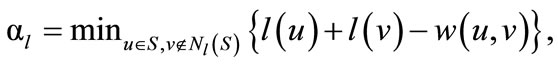
The Kuhn-Munkres theorem transforms the problem from an optimization problem of finding a maximum weight matching into a combinatorial one of finding a perfect matching. Thus, the Hungarian algorithm is devised by starting with any feasible labeling l and some matching M in El. and repeating the following while M is not perfect:
1) Find an augmenting path for M in El;
2) If no augmenting path exists, improve l to  such that
 ; Go to 1).
Note that in each step of the loop we will either be increasing the size of M or El so this process must terminate. Furthermore, when the process terminates, M will be a perfect matching in El for some feasible labeling l. Hence, M will be a maximum weight matching.
3. Symbolic Formulation
An ordered binary decision diagram (OBDD) [6,7] provides compact, canonical and efficiently manipulative representation for Boolean functions. The OBDD for a non-constant Boolean function f is a directed acyclic graph . It includes sink or terminal nodes ‘0’ and ‘1’, which represent constant Boolean functions 0 and 1. These nodes have no descendants. All other nodes
  include a labeled variable
 , and have two out-going edges of then and else cofactors drawn as solid and dash lines. The nodes are in one-to-one correspondence with Boolean functions. The function
  of a node
  is specified as
 where “×” and “+” denote Boolean conjunction and disjunction respectively, and
  and
and  are the functions of the then and else children. The root node of an OBDD represents the function f. The variables in an OBDD are ordered, i.e., if v is a descendant of u, which means
 , then
 , and all the paths in the OBDD keep the same variable ordering.
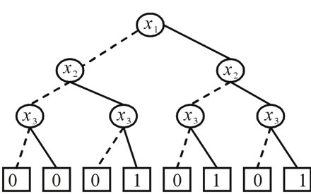
Given a Boolean function and any assignments to its variables, the function value is determined by tracing a path from the function node to a terminal node following the appropriate branches. The branches depend on the variable value of the assignments, and the function value under the assignments is determined by its path’s terminal or sink node.
For example, Figure 1 shows the binary tree and the OBDD for Boolean function , where
 . It is obvious that the OBDD is a directed acyclic graph, and stores the same information in a more compact way. We trace the path ®‚®ƒ®„, and reach the sink node 0. Thus, the value of Boolean function
  of variable assignment (0,1,0) is 0.
A set is a non-order collection of elements with any specified properties. A set is perhaps the most fundamental mathematical abstraction and can be seen as a generic concept to build various representations of discrete objects. We can convert a set S to an OBDD by encoding the elements of S with a length-n binary number, where . The encoded element in S corresponds to a vector of binary variables
 .
.
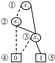
Thus, a set S can be formulated by the following Boolean characteristic function:
 (4)
(4)
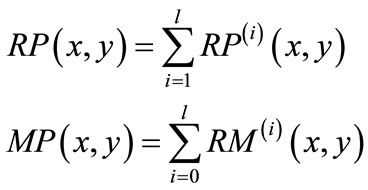
where  is the appearance of variable xk corresponding to k bit code of the s-th element of set S. Set operations can be reduced to the operations on Boolean characteristic functions as follows:
union of sets: 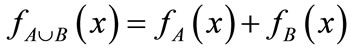
intersection of sets: 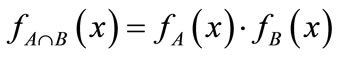
difference of sets: 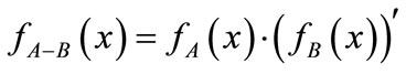
A relation is a set of ordered pairs. Given a relation R from A to B, we can formulate the relation as an OBDD by encoding the elements of A with a length-n binary number and the elements of B with a length-m binary number, where 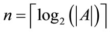 and
and .
.
The encoded element in A corresponds to a vector of binary variables , and the encoded element in B to a vector of binary variables
 . Therefore, a pair (a, b) in R can be formulated by the following Boolean characteristic function:
 (5)
(5)
where  is the appearance of variable
  corresponding to k bit code of element
 , and
, and  the appearance of variable
  corresponding to k bit code of element
 . If
. If , then
 , else
 . Similarly, If
 , then
 , else
 . The relation R can be formulated as:
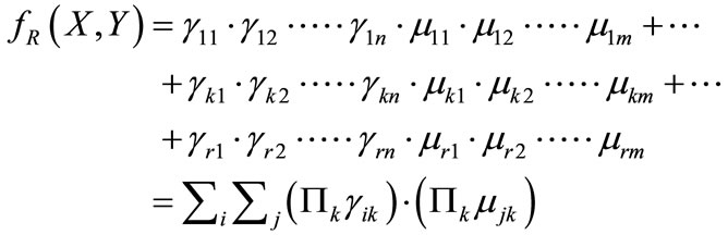 (6)
(6)
where  is the appearance of variable xk corresponding to k bit code of the i-th element of set A, and mik the appearance of variable yk corresponding to k bit code of the j-th element of set B. If
 , then
 , else
 . Similarly, If
 , then
 , else
 .
.
These characteristic functions are of Boolean functions, and can be compactly represented by OBDDs. For example, the characteristic functions of set  and set
  are derived by encoding
 ,
,  ,
,  , d = [011],
  ,
,  and
and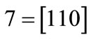 :
:

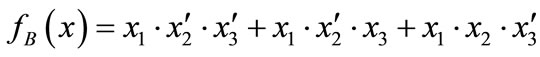
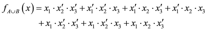
The characteristic function of relation R = {(a,1), (a,5), (b,1), (b,7), (c,1), (c,5), (d,7)} is derived by encoding ,
,  ,
,  ,
,  ,
,  ,
,  and
and :
:
The OBDDs for these characteristic functions are shown in Figure 2.
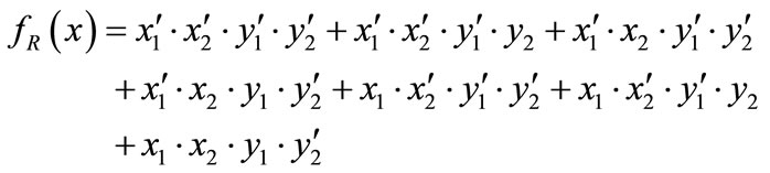
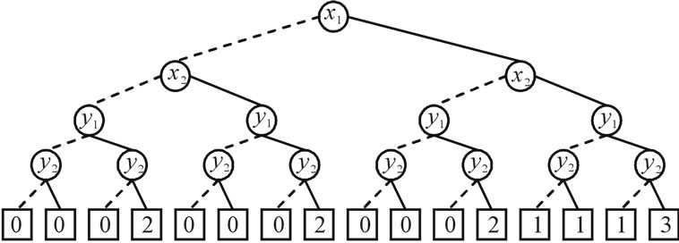
An algebraic decision diagram (ADD) [12] is a variant of OBDD, representing pseudo-Boolean functions , where S is the finite carrier of the algebraic structure. The only difference of an ADD from an ODD is that each terminal node of an ADD represents constant function corresponding to the finite carrier. When the finite carrier is set to
 , an ADD is reduced to an OBDD. For example,
  , where
 . Figure 3 shows the complete binary tree and the ADD for f. We can also see that the ADD for f is a directed acyclic graph that stores the same information in a more compact way.
ADDs are a natural symbolic representation of matrices since every r ´ s matrix W can be represented by a pseudo-Boolean function fW(x, x):
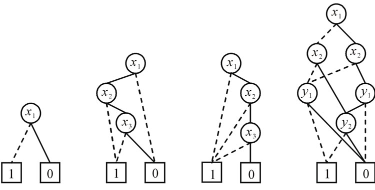
Figure 2. OBDD formulation of sets and relation.
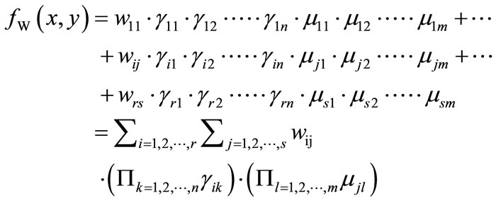 (7)
(7)
where  is the element at the i-th row and the i-th column in matrix W;
  is the appearance of variable
  corresponding to k bit code of i
  , and
, and  the appearance of variable yk corresponding to l bit code of j
  . If
. If , then
 , else
 . Similarly, If
 ,then
,then , else
  .
.
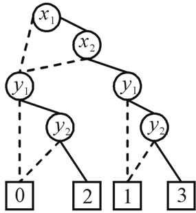
For example, the following 4 × 4 matrix
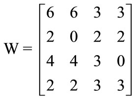
can be represented symbolically by encoding row number as 00,01,10 and 11, and column number as 00,01,10 and 11. Its pseudo-Boolean function fW(x,y) can be derived from Equation (7):
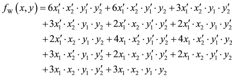
The ADD for this matrix is drawn in Figure 4.
Given a weighted bipartite graph , we can encode the nodes of G with a length-n binary number, where
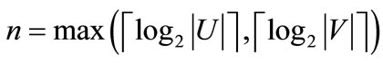 , and represent the nodes in U as a vector of binary variables
 , and the nodes in V as a vector of binary variables
 . The edge
  can be formulated by a binary vector
 , where x = encoded
  and y = encoded
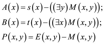
  are the binary encoding of node u and v respectively. In terms of Equations (4) (6) and (7), the Boolean or pseudo-Boolean characteristic functions of its elements can be developed, and denoted by s(x), t(y), E(x, y) and W(x, y) for node set U, node set V, edge set E and weight function W respectively.
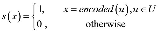 (8)
(8)
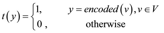 (9)
(9)
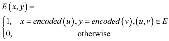 (10)
(10)
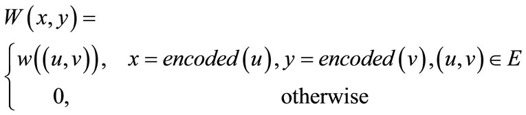 (11)
(11)
For example, Figure 5 illustrates a weighted bipartite graph, whose weight function or edge weights are specified in the weight matrix. Nodes in U can be encoded by (00, 01, 10, 11) and nodes in V can be encoded by (00, 01, 10, 11). In terms of Equations (10) and (11), OBDD for E(x, y) and ADD for W(x, y) are developed and shown in Figure 5.
An important property of OBDDs or ADDs is that they are a canonical representation of Boolean functions or pseudo-Boolean functions. Canonicity means that for a Boolean function or pseudo-Boolean function f and
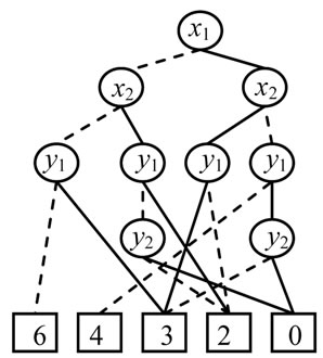
Figure 4. Representing a matrix by ADD.
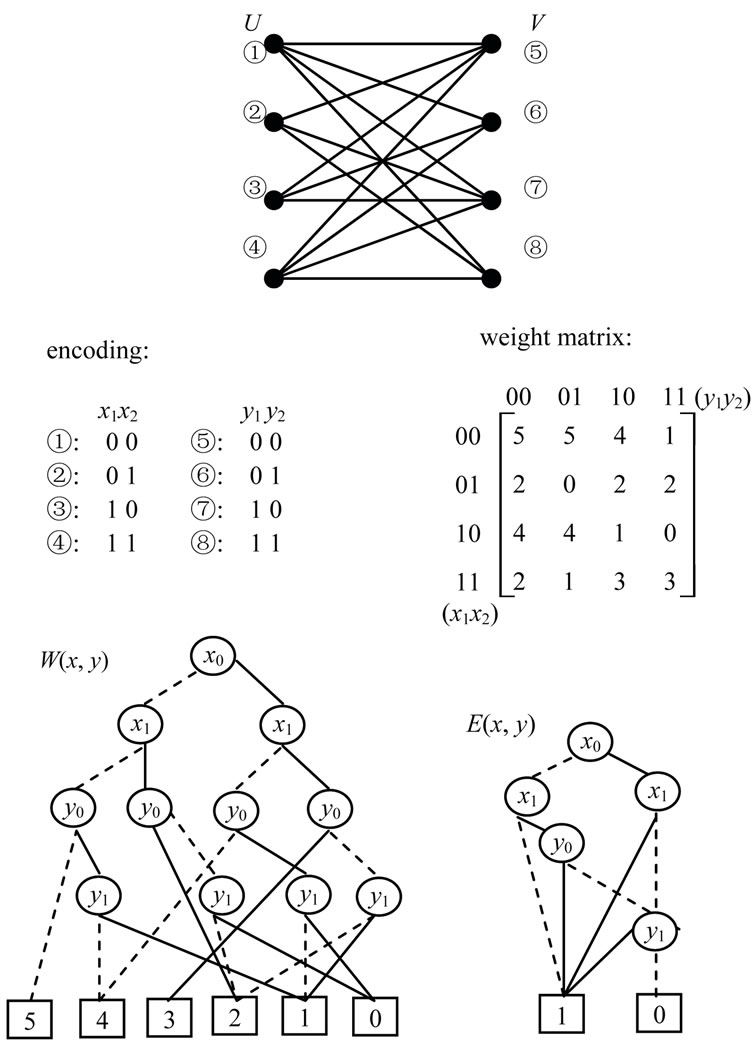
Figure 5. Symbolic representation of a weighted bipartite graph.
variable ordering p, there is a unique OBDDs or ADDs, and vice versa. It is more important that many operations of Boolean functions or pseudo-Boolean functions can be implemented efficiently through graphical manipulations of OBDDs or ADDs.
Given a weighted bipartite graph  or its symbolic formulation (s(x), t(y), E(x,y), W(x,y)), finding the maximum weighted matching M(X, Y) in bipartite graphs is formulated as follows:
max:
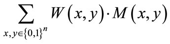 (12)
(12)
subject to:
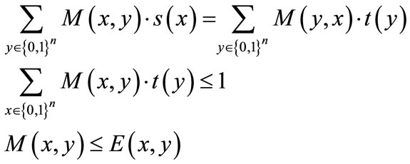 (13)
(13)
4. Symbolic ADD Algorithm
Given the symbolic representation (s(x),t(y),E(x,y),W(x,y)) of a weighted bipartite graph , the pseudo-code of the symbolic ADD algorithm for maximum weighted matching is presented in Figure 6.
The symbolic algorithm implements the Hungarian algorithm in the context of ADD and OBDD formulation and manipulations. It begins by setting feasible labelings of nodes and then iterates through a sequence of phases. Each phase is divided into two stages. The first stage is building equality bipartite graphs, and the second one is finding maximum cardinality matching in equality bipartite graphs. The second stage iterates through following steps: greedily searching initial matching; building layered network, backward traversing node-disjoint augmenting paths, updating cardinality matching and building residual network. The second stage terminates and returns the maximum cardinality matching when there does not exist any augmenting path of equality bipartite graph. The symbolic algorithm stops and returns the maximum weighted matching when there does not exist any augmenting path in weighted bipartite graph.
4.1. Building Equality Bipartite Graphs
Given a weighted bipartite graph with a feasible labeling l, represented as ((s(x),t(y),E(x,y),W(x,y)), l(x), l(y)), we define two  auxiliary matrices: the first one is developed by arranging the vector of l(y) column by column, and the second one is created by arranging the vector of l(x)T rank by rank. We denote them by corresponding characteristic functions Al(y)(x,y) and Al(x)(x,y). The equality bipartite graph is built as follows:
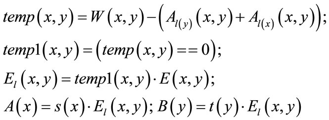 (14)
(14)
The equality bipartite graph is represented as (A(x), B(y), El(x,y)), in which A(x) and B(y) are the disjoint node sets, and will be utilized to control the progress of searching direct matching and building layer networks in the later phases.
In order to update a feasible labeling l, we introduce the neighbor of  and set
 :
:
 ,
,
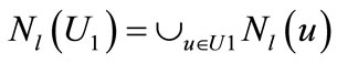
They can be computed and represented by the following characteristic functions:
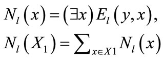 (15)
(15)
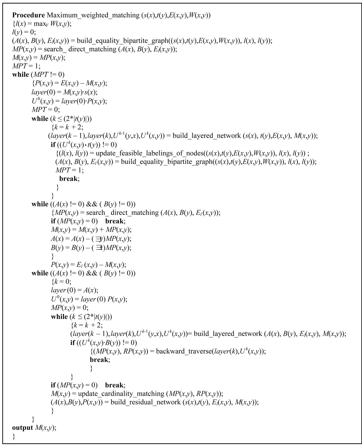
Figure 6. Pseudo-code for symbolic algorithm.
Then, a feasible labeling l is updated by the following feasible labeling l¢:
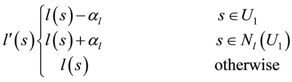 (16)
(16)
4.2. Searching Matching through Proximity Functions
In order to obtain matching directly, we adopt a proximity function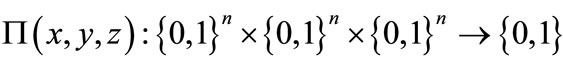 . The first argument is the base, and two other arguments are the nodes to be compared. For every choice of base X, P returns 1 if the second argument precedes the third one, else return 0.
Two different heuristic functions are used in the symbolic algorithm. The first one, relative proximity heuristic function, is 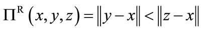 , where
 . The second is
 , called as datum proximity heuristic function that is a special case of relative proximity heuristic function independent of the base and simply returns the result of testing
 . Both proximity functions can be represented by BDDs of size linear in n [14].
We obtain a direct matching of bipartite graph (s(x), t(x), E(x, y) ) by the following computation:
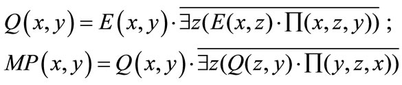 (17)
(17)
The edges in Q(x,y) form a right-unique relation, i.e., there is at most one edge out of each node x. MP(x,y) is a left-unique subset of Q(x,y), and consists of edges that share no end nodes. For example, Figures 7(b) and (c) show the initial matching (darkened lines) of the bipartite graph in Figure 7(a) using relative proximity function and datum proximity function respectively. The proximity functions are also applied in finding node-disjoint augmenting paths. We will discuss it below.
4.3. Building Layered Network
On finding the initial matching, we need to build a layered network so as to obtain node-disjoint augmenting paths. We initialize layer zero by nodes layer(0) of unmatched nodes in s(x) and outgoing edges  of unmatched edges from layer(0). On odd layer
 , nodes layer
 are target-nodes from edges
  (x,y), and outgoing edges
  include the matched edges from layer
 . Even layer
  has nodes layer(2i) of target-nodes from edges
 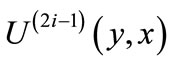 and outgoing edges
 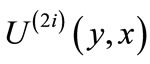 of unmatched edges from layer(2i). A layered network is created by forward-breadth-first traversing residual network. It is implemented by the following computations:
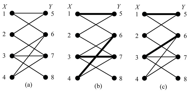
Figure 7. Finding direct matching by proximity function.
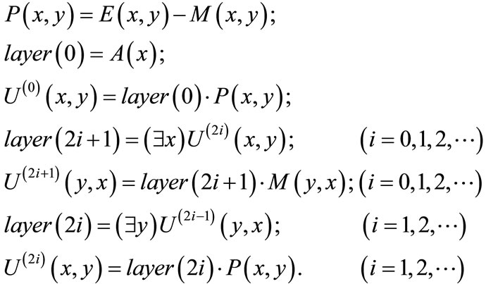 (18)
(18)
4.4. Backward Traversing Node-Disjoint Augmenting Paths
Once a layered network is constructed, we go through a series of steps to find node-disjoint augmenting paths. Supposed that the top layer of layered network with k = 2l layers satisfies  != 0, i.e.,
  will have unmatched nodes, we proceed to build nodedisjoint augmenting paths backward from unmatched edges
  and matched edges
 :
:
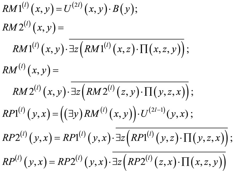 (19)
(19)
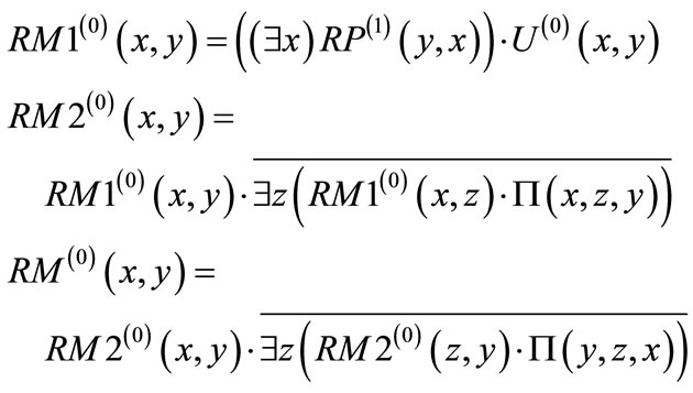
Backward breadth-first traversing is implemented by the following computations (where i = (l – 1), (l – 2),…,2, 1.):
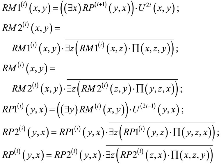 (20)
(20)
This process terminates by computing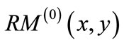 resulting in node-disjoint
 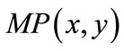 and
and . Proximity functions guarantee that the augmenting paths are node-disjoint and have the shortest length.
 (21)
(21)
 (22)
(22)
4.5. Updating Cardinality Matching and Building Residual Network
Matching is updated by adding unmatched edges 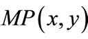 and deleting matched edges
 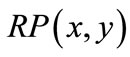 of node-disjoint augmenting paths:
 (23)
(23)
The algorithm is continued by searching residual network repeatedly till there is no augmenting path. A residual network is symbolically formulated by ,
,  ,
,  and
and :
:
 (24)
(24)
Since the symbolic algorithm is based on ADD and OBDD formulations and operands, edges or vertices are enumerated implicitly, and the edge-disjoint paths are traced in parallel. Nevertheless, the symbolic algorithm is developed in the framework of Kuhn-Munkres algorithm, and we can make a claim that its time complexity is .
.
5. Experimental Results
The symbolic algorithm proposed in this paper has been implemented in windows 2000 and software package CUDD [17]. Two groups of experiments are conducted. In both cases, CPU time is in second on a P4 1500 MHz with 128 MB of memory.
In the first group of experiments, the symbolic algorithm (SA) is compared with KMA and CSA algorithms [3]. We choose randomly generated graphs with different numbers of nodes and edges. Random graphs are very close to worst cases for symbolic algorithms. The results are shown in Table 1. In the second group of experiments, we choose randomly generated graphs with 2500 nodes and different ranges of edge weights, and our symbolic algorithm is compared to CSA algorithm. The running times are plotted in Figure 8.
Both the symbolic algorithm and traditional algorithms utilize the input of normal weighted bipartite graph . The SA package calls the CUDD library to create the symbolic formulation (s(x), t(y), E(x,y), W(x,y)) and implement Kuhn-Munkres algorithm. The traditional algorithms are implemented using LEDA package [18].
Both groups of experiments indicate that symbolic algorithm outperforms both KMA and CSA algorithms, especially on dense and large random graphs. It can also be observed that the running times of our symbolic algorithm increase as the ranges of edge weights increase.
6. Conclusions
We present an algorithm for finding the maximum weighted matching in bipartite graphs. The algorithm is symbolic and does not require explicit enumeration of
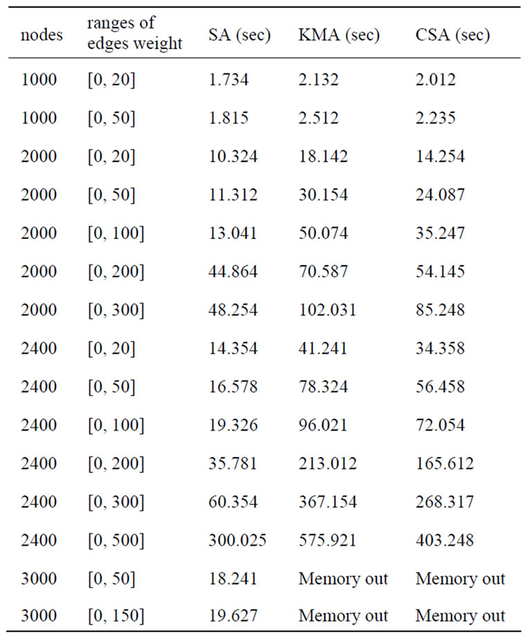
Table 1. Comparison of symbolic algorithm with KMA and CSA algorithms.
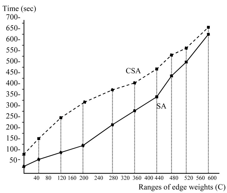
Figure 8. Comparison of symbolic algorithm to CSA for graphs with varying ranges of edge weights.
the nodes and edges of the graphs. The main idea is to manipulate implicitly sets of edge-disjoint augmenting paths, in which the disjointness is enforced with the help of priority functions. Since all paths in a maximal edgedisjoint set are traced in parallel, the algorithm can handle much larger graphs than it was previously possible. It should be stressed that algorithms that explicitly enumerate edges or vertices cannot be applied to very large problems. We have also shown that the algorithm is competitive with traditional algorithms on dense random graphs.
Several aspects of the work we have presented require further investigation. We should be able to further improve performance by applying more sophisticated OBDD and ADD techniques (e.g., variable ordering, caching). More important, we should be able to deal with substantially larger graphs. Further enhancements to the algorithm may come from improved priority functions. We have chosen path augmentations as the basis of our algorithm. Whether efficient symbolic versions of preflowbased algorithms can be found remains an interesting open question. Another open question concerns the complexity of the algorithm. In particular, a characterization only in terms of worst-case run times is unsatisfactory for symbolic algorithms. We are also working on extending our algorithm to general graphs. Moreover, it is clear that the principles behind the symbolic matching algorithm can be applied to many other problems in various areas.
7. References
[1] R. K. Ahuja, T. L. Magnanti and J. B. Orlin, “Network Flows: Theory, Algorithms, and Applications,” Pearson Education Inc., Prentice Hall, Englewood Cliffs, 1993.
[2] Z. Galil, “Efficient Algorithm for Finding Maximum Matching in Graphs,” ACM Computing Surveys, Vol. 18, No. 1, 1986, pp. 23-37. doi:10.1145/6462.6502
[3] H. W. Kuhn, “The Hungarian Method for Assignment Problem,” Naval Research Logistics Quarterly, Vol. 2, No. 1-2, 1955, pp. 83-97. doi:10.1002/nav.3800020109
[4] J. Munkres, “Algorithms for Assignment and Transportation Problems,” Journal of SIAM, Vol. 5, No. 1, 1957, pp. 32-38.
[5] H. N. Gabow and R. E. Tarjan, “Faster Scaling Algorithms for Network Problems,” SIAM Journal on Computing, Vol. 18, No. 5, 1989, pp. 1013-1036. doi:10.1137/ 0218069
[6] A. V. Goldberg, S. A. Plotkin and P. M. Vaidya, “Sublinear Time Parallel Algorithms for Matching and Related Problems,” Journal of Algorithms, Vol. 14, No. 2, 1993, pp. 180-213. doi:10.1006/jagm.1993.1009
[7] J. B. Orlin and R. K. Ahuja, “New Scaling Algorithms for the Assignment and Minimum Cycle Mean Problems,” Sloan Working Paper 2019-88, Solan School of Management, Massachusetts Institute of Technology, Cambridge, 1988.
[8] A. V. Goldberg and R. Kennedy, “An Efficient Cost Scaling Algorithm for the Assignment Problem,” Mathematical Programming, Vol. 71, No. 2, 1995, pp. 153- 178. doi:10.1007/BF01585996
[9] R. E. Bryant, “Graph-Based Algorithms for Boolean Function Manipulation,” IEEE Transactions on Computer, Vol. 35, No. 8, 1986, pp. 677-691. doi:10.1109/TC.1986. 1676819
[10] R. E. Bryant, “Symbolic Boolean Manipulation with Ordered Binary Decision Diagrams,” ACM Computing Surveys, Vol. 24, No. 3, 1992, pp. 293-318. doi:10.1145/13 6035.136043
[11] S. B. Akers, “Binary Decision Diagrams,” IEEE Transactions on Computer, Vol. 27, No. 6, 1978, pp. 509-516. doi:10.1109/TC.1978.1675141
[12] D. Sieling and R. Drechsler, “Reduction of OBDDs in Linear Time,” Information Processing Letters, Vol. 48, No. 3, 1993, pp. 139-144. doi:10.1016/0020-0190(93)90 256-9
[13] D. Sieling and I. Wegener, “Graph Driven BDDs: A New Data Structure for Boolean Functions,” Theoretical Computer Science, Vol. 141, No. 1-2, 1995, pp. 283-310. doi: 10.1016/0304-3975(94)00078-W
[14] G. D. Hachtel and F. Somenzi, “A Symbolic Algorithm for Maximum Flow in 0-1 Networks,” Formal Methods in System Design, Vol. 10, No. 2-3, 1997, pp. 207-219. doi:10.1023/A:1008651924240
[15] R. I. Bahar, E. A. Frohm, C. M. Gaona, et al. “Algebraic Decision Diagrams and Their Applications,” Formal Methods in Systems Design, Vol. 10, No. 2-3, 1997, pp. 171- 206. doi:10.1023/A:1008699807402
[16] T. L. Gu and Z. B. Xu, “The Symbolic Algorithms for Maximum Flow in Networks,” Computers & Operations Research, Vol. 34, No. 2, 2007, pp. 799-816. doi:10.101 6/j.cor.2005.05.009
[17] F. Somenzi, “CUDD: CU Decision Diagram Package Release 2.3.1,” 2006. http://vlsi.Colorado.edu/
[18] The LEDA User Manual, 2010. http://www.algorithmicsolutions.com
NOTES
*This work was supported in part by National Natural Science Foundation of China (60963010, 60903079) and Key Natural Science Foundation of Guangxi Province (0832006Z).