Journal of Water Resource and Protection
Vol.5 No.11(2013), Article ID:40081,11 pages DOI:10.4236/jwarp.2013.511110
Numerical Simulation of Unsteady Friction in Transient Two-Phase Flow with Godunov Method
1Department of Civil, Geological and Mining Engineering (CGME), Polytechnique Montreal, Succursale Centre, Ville Montréal, Canada
2Department of CGME, Polytechnique Montreal, Succursale Centre, Ville Montréal, Canada
Email: samba.bousso@polymtl.ca, musandji.fuamba@polymtl.ca
Copyright © 2013 Samba Bousso, Musandji Fuamba. This is an open access article distributed under the Creative Commons Attribution License, which permits unrestricted use, distribution, and reproduction in any medium, provided the original work is properly cited.
Received March 11, 2013; revised April 13, 2013; accepted May 12, 2013
Keywords: Finite Volume; Godunov Method; Transient Flow; Two Phase Flow; Unsteady Friction
ABSTRACT
Most numerical transient flow models that consider dynamic friction employ a finite differences approach or the method of characteristics. These models assume a single fluid (water only) with constant density and pressure wave velocity. But when transient flow modeling attempts to integrate the presence of air, which produces a variable density and pressure-wave velocity, the resolution scheme becomes increasingly complex. Techniques such as finite volumes are often used to improve the quality of results because of their conservative form. This paper focuses on a resolution technique for unsteady friction using the Godunov approach in a finite volume method employing single-equivalent twophase flow equations. The unsteady friction component is determined by taking into account local and convective instantaneous accelerations and the sign of both convective acceleration and velocity values. The approach is used to reproduce a set of transient flow experiments reported in the literature, and good agreement between simulated and experimental results is found.
1. Introduction
Friction in pressurized flows can be decomposed into two components: static friction in steady flows and dynamic friction in transient flows. Transient flows present fairly important dynamic frictions that can significantly modify system behavior. Several types of model are used to calculate the dynamic friction component. One of the first types is the convolution-based model developed by Zielke [1], which uses the local acceleration and weight functions to calculate the unsteady friction component for laminar flow. The integration procedure in the Zielke model requires lots of memory and is very time-consuming. Others such as Suzuki et al. [2] and Schohl [3] suggested improvements in the determination of the unsteady friction component. Later, Vardy and Brown [4,5], Prashanth Reddy et al. [6] and Vitkovsky et al. [7] proposed an extension of the Zielke convolution model for smooth and rough pipes with turbulent flow. Another type of model called the instantaneous accelerations-based model is noted in the literature. It attributes the attenuation of flow amplitudes to local  and convective instant acceleration
  [6,8,9]. In instantaneous accelerations-based model, the friction coefficient
  is decomposed into a static friction component
  and an unsteady friction component
  (Equation (1)).
 (1)
(1)
with:
 (2)
(2)
where  is the Brunone coefficient,
  is the pipe diameter,
  is the water velocity,
  is the pressure wave celerity,
  is the time and
  is the abscissa.
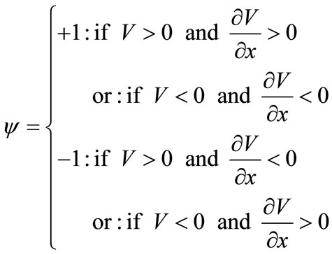
Bergant et al. [10] improved this formulation by introducing  instead of
 , to better reproduce the attenuation of flow acceleration and deceleration. For producing good accuracy in case of an upstream valve closing, second improvement was considered by the sign of the velocity and its acceleration or deceleration
  [11-13].
For solving transient flows with the dynamic friction, several numerical methods are proposed in the literature and two approaches are generally used. The first approach involves calculating the local and convective acceleration in the source term  (see Equation (4)) as treated by Bergant et al. [10], Brunone et al. [14] and Bughazem and Anderson [15]. The second one transfers acceleration or one part of acceleration in the variables and the flux terms (see Equation (4)), as illustrated by Bughazem and Anderson [16], Wylie [17] and Vítkovský et al. [11]. The first approach uses finite differences, while the second employs the method of characteristics that is a graphical procedure for the integration of partial differential equations (PDEs) [18]. Prashanth Reddy et al. [6] used the second type of resolution with the characteristic equations developed by Vitkovsky et al. [11] to calculate the dynamic friction component. The formulation of the dynamic friction component in the instantaneous accelerations-based model has been tested with finite difference techniques and the method of characteristics. However, there is a lack of literature on the use of the finite volume technique in instantaneous accelerationsbased models.
Finite volume techniques, particularly those using the Godunov method (as presented by Toro [19] and Guinot [20]) are now widely used for transient flow in sewers (as in León et al. [21], Vasconcelos and Wright [22] and Sanders and Bradford [23]) but without unsteady friction. This paper presents and applies the instantaneous accelerations-based model including a numerical method based on Godunov approach. Four specific objectives are targeted: i) to modify the single equivalent two-phase flow equations, ii) to consider air content, i.e. some compressibility, in the equations, iii) to propose a numerical method, and iv) to compare numerical and experimental results.
2. Methodology
The first section of the paper proposes the governing equations and the second a numerical method adapted from Guinot’s [20] traffic flow model. The third section presents two case studies in which numerical and experimental results are analyzed. The proposed model is governed by the single-equivalent two-phase flow equations. The dynamic friction component refers to the instantaneous accelerations-based model formulation and the resolution scheme uses the Godunov approach. This formulation of equations considers some compressibility of the fluid with variable density and pressure wave celerity. The model results are compared to experimental measurements from Adamkowski and Lewandowski [24] and Bergant et al. [25].
3. Governing Equations
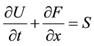
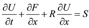
The pressurized flow Equations (3) and (4) are those presented by Guinot [20] for the calculation of waterhammer in the presence of a two-phase fluid with an air content.
 (3)
(3)
Vectors ,
,  and
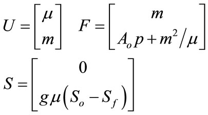
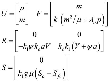
and  correspond, respectively, to the variables, flux and source term defined by Equation (4).
 (4)
(4)
where:  and
and  represent the time and the abscissa,
  the flow cross-section,
  the flow discharge,
  the fluid density,
  the mass of fluid per unit length of the pipe,
  the mass discharge,
  the pressure,
  the pipe slope,
  the friction slope calculated by Dary-Weisbach formula as following
 ,
,  acceleration of gravity, and
  the water velocity.
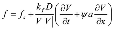
The friction coefficient is determined by considering local and convective instantaneous accelerations as in the model by Brunone et al. [8,9] that was modified by Bergant et al. [10] as in Equation (5).
 (5)
(5)
where the Brunone coefficient  depends on
  expressed in Equation (6).
 (6)
(6)
Friction  is therefore first decomposed into static
  and dynamic
  components as shown in Equation (5). The dynamic friction component is transformed according to the variables flow
  and
and  in Equation (7):
 (7)
(7)
In which:
 (8)
(8)
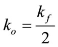
The Brunone coefficient  is determined as in Bergant et al. [10] by:
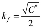 (9)
(9)
where  (Equation ) depends more on the flow regime (Reynolds number
 ).
).
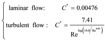 (10)
(10)
The contributions of the dynamic friction acceleration  in the vector variable
  and in the flux vector
  (Equation (4)) allows to obtain Equation (11), in which
  is the friction slope due to the dynamic friction component.
 (11)
(11)
In vectorial form Equation (11) become Equation (12), where the sought variables are  and
and . The other variables
  will be determined by considering the Equations (24), (25) and
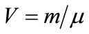 .
.
 (12)
(12)
with:
 (13)
(13)
and
 (14)
(14)
Equations (12) and (13) are equivalent to Equations (3) and (4) if the dynamic friction component is not considered (i.e., ).
).
The next proposes a numerical method for solving these equations for each internal cell. The exterior cells will be determined by the boundary conditions formalized in each case. Since a variable is known for each pipe end, one of the Riemann invariants will be used to calculate the second variable. For example, for a known discharge or pressure to the left boundary, the second Riemann invariant is used to calculate the second variable (discharge or pressure). When it is the right boundary, the first Riemann invariant is used. Details of the calculation will be discussed in the next section.
4. Procedure for Numerical Solution of Partial Differential Equations (PDEs)
Equations (12) and (13) resemble the Guinot’s [20] traffic flow model, in which the acceleration/deceleration of a vehicle influences the speed of the preceding vehicle. Solving this non-conservative system of balance equations with the Godunov approach by using the solution of the Riemann problem, involves four steps:
The first step is to make the solution of the Riemann problem of Equation (15) to express the conservation component of Equation (12):
 (15)
(15)
The second is to analyze the solution of the Riemann problem of the second hyperbolic part (Equation (16)):
 (16)
(16)
The third is to obtain the solution of the Riemann problem of the source term  corresponding to Equation (17):
 (17)
(17)
The fourth step is to obtain all parameters (as velocity  and pressure
  in each cell) needed to determine the flow. The next time
  step is calculated by taking into account the Courant condition:
 ,
,  corresponding to the spatial step.
4.1. Step 1: Solution of the Riemann Problem for the Conservation Part
The conservative part is close to the two-phase flow of the equation presented by Guinot [20] and León et al. [21]. The only difference is the factor  in the second line of the flux
  regarding Equation (13). If the dynamic friction component (i.e.,
 ) is not considered, the equations are those usually used when only the static friction component is considered. Considering
 , the Jacobian matrix of
  respecting the matrix
 ,
,  can be found in Equation (18):
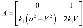 (18)
(18)
After processing and arrangement, the eigenvalues of the matrix  are given by Equation (19).
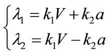 (19)
(19)
With:
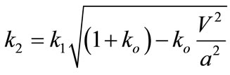 (20)
(20)
The eigenvalues, corresponding to the eigenvectors for the matrix , are
, are  and
and  as seen in Equation (21).
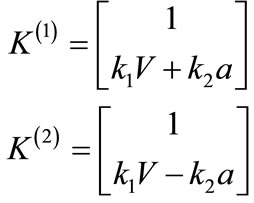 (21)
(21)
4.1.1. Riemann invariants of the Conservative Solution
The Riemann invariants along each characteristic  are given by Equation (22).
 (22)
(22)
Equation (22) can be integrated respectively between  and
and  following approximation according to the trapezoidal rule, as with static friction.
  represents the variables to the left of the region of the constant state,
  the region of the constant state and
  those to the right of the constant state region. The resulting equation (Equation (23)) is solved by the Newton Raphson method for determining
  i.e.
i.e.  and
and .
.
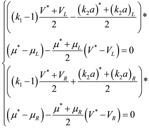 (23)
(23)
Note that the celerity , which depends on
 , is related to other parameters through Equation (24), as presented by Guinot [26].
 (24)
(24)
With  fluid density,
  the volume fraction of air at the reference pressure
 ,
,  the polytropic coefficient of air (
 for isothermal conditions and
  for adiabatic conditions). The pressure waves celerity
  in water is calculated as suggested by Wylie and Streeter [27].
The solution of Equation (23) yields:  and
and  i.e.
i.e.  and
and  used for calculating the mass discharge
  and the vector variable
 . The pressure force
  is obtained by solving Equation (25) [20].
 (25)
(25)
4.1.2. Boundary Conditions Calculation of the Conservative Part
The approach assumes half-virtual cells at  and
and  as suggested by Guinot [20], using a reference pressure/velocity depending on the boundary conditions type.
Prescribed pressure at the left boundary
If the pressure is prescribed, i.e. known at the left boundary, then Equation (25) is used to determine . Therefore Equation (24) can be used to determine
  from
from . The Riemann invariant along
  (Equation (23)) yields the velocity
 (Equation (26)) with
  corresponds to flow parameter
  at cell 1 at time
 .
.
 (26)
(26)
Prescribed discharge at the left boundary
If the discharge is known, then the velocity Riemann invariant (Equation (27) along
 is combined with Equations (24) and (25) yields
  and
and .
.
 (27)
(27)
Prescribed pressure at the right boundary
If the pressure is prescribed at the right boundary, Equations (25) and (24), and Riemann invariant along  (Equation (28) or (29)) provide
  and
and  with
with  corresponding to flow parameter
  at cell
  at time
 .
.
 (28)
(28)
 (29)
(29)
Prescribed discharge at the right boundary
When discharge  is prescribed, Riemann invariant (Equation (28)) along
 , combined with Equations (24) to (25), yields
 ,
,  and
and  as shown in Equation (30):
 (30)
(30)
4.1.3. Balance over the Cells
The conservative part yields the homogeneous solution (Equation (31)) at each cell without the source term as presented by Guinot [20]:
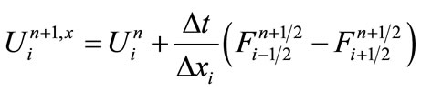 (31)
(31)
The flux  will be calculated by Equation (32):
 (32)
(32)
The provisional values  will be corrected in two successive stages, integrating the second hyperbolic part
  and the source term
 .
.
4.2. Step 2: Solution of the Riemann Problem of the Second Hyperbolic Part
Equation (16) is solved by seeking the eigenvalues and vectors of  (Equations (33)).
 (33)
(33)
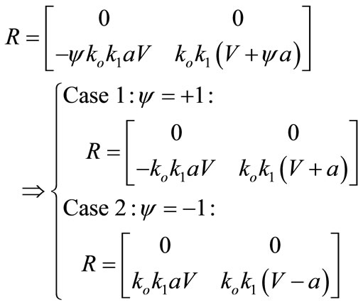
Given that eigenvalues and vectors of  differ depending on the sign of
 , each case of Equations (33) is treated separately in sections 4.2.1 for
  and in section 4.2.2 for
 .
.
4.2.1. Resolution of Case 1
Eigenvalues and eigenvectors of  for Case 1 are depicted in Equations (34) and (35), respectively:
 (34)
(34)
 (35)
(35)
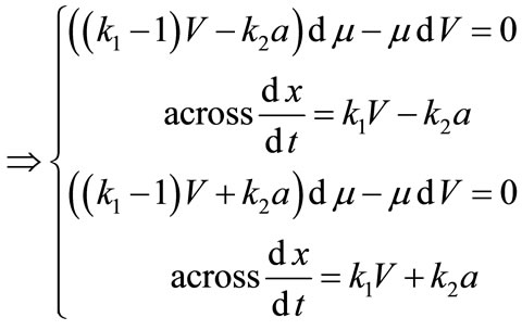
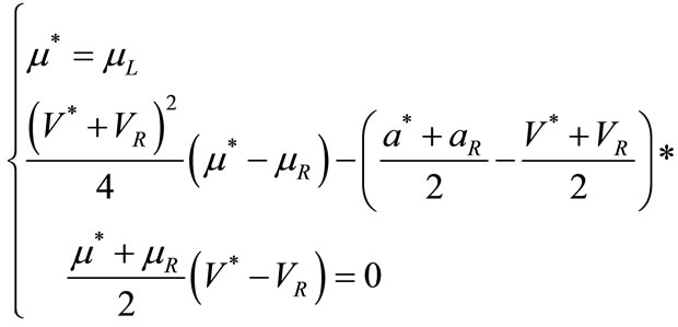
Considering the validity of the eigenvectors in Equation (35), along each characteristic line, solution of the Riemann problem (Equation (36)) is obtained.
 (36)
(36)
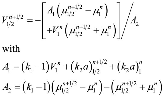
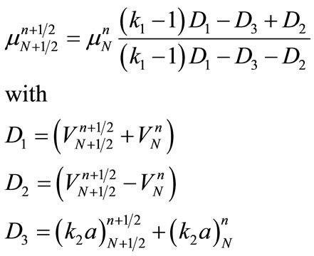
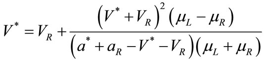
Using the trapezoidal rule, as in Equation (37), the velocity  of the constant state is calculated by Equation (38).
 (37)
(37)
 (38)
(38)
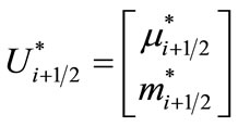
After the determination of  and
and , the vector variable
  is determined for each inter face. The new variable
  considering the second hyperbolic part is then calculated by applying the Riemann invariants principle [19,20]:
 (39)
(39)
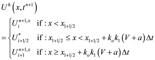
4.2.2. Balance over the Cells
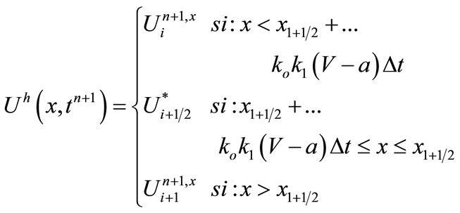
The following formulation (Equation (40)) is obtained when  is integrated over the cell for
 .
.
 (40)
(40)
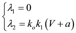
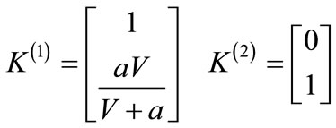
4.2.3. Resolution of Case 2
In Case 2 , eigenvalues (
 and
and ) and eigenvectors (
 and
and ) of
) of  are respectively Equations (41) and (42):
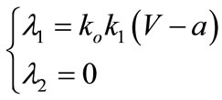 (41)
(41)
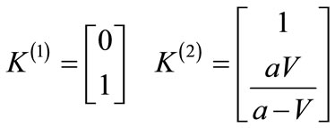 (42)
(42)
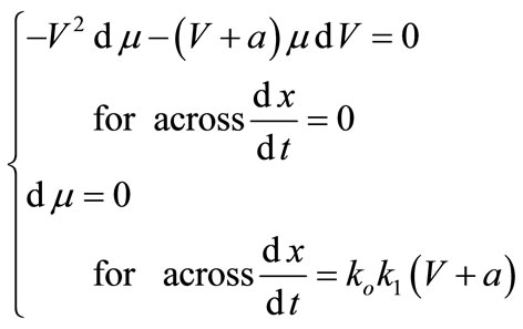
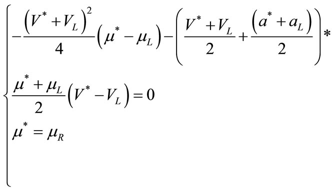
As in Case 1, the Riemann invariant is expressed by Equation (43).
 (43)
(43)
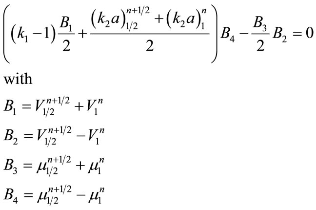
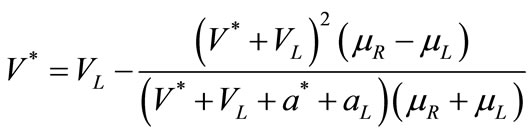
The second part of the solution of the Riemann problem (Equation (43)) is used to calculate the velocity  of the constant state (Equation (44) or (45)).
 (44)
(44)
 (45)
(45)
The quantities  and
and  yield the vector variable
 .
.
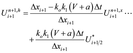
The new variable  taking into account the second hyperbolic part is then calculated by applying the principle of Riemann invariants:
 (46)
(46)
4.2.4. Balance over the Cells
Integrating Equation (46) over the cell yields  for
for :
:
 (47)
(47)
4.2.5. Boundary Conditions
The last cell is calculated by considering either the first component of Equation (37) for  or the second component of Equation (44) for
 . Each of the resulting Equations (48) or (49) is combined with the known flow condition:
 (48)
(48)
 (49)
(49)
with  dependant respectively on
  and
and .
.
4.3. Step 3: Solution of the Riemann Problem of the Source Term
The source term is solved by Equation (50) to estimate the variable vector  of each cell depending on
 , as presented by Guinot [20] and Toro [19].
 (50)
(50)
where  indicates that
  is used to evaluate the source term
  of the Equation (13).
4.4. Step 4: Flow Parameter Calculation
After determining the variables  and
and , velocity
 , density
 , pressurewave celerity
  by Equation (24), and pressure
  by Equation (25) are determined for each cell.
5. Results and Discussion
Two case studies ((1) a closed downstream valve and (2) a closed upstream valve) are performed, and numerical results compared to the experimental results.
5.1. Case Study 1: Closed Downstream Valve Analysis
5.1.1. Experimental Setup of the Case Study 1
The used experimental results are from the study of Adamkowski and Lewandowski [24]. The experiments were conducted at a test rig composed of a 98.11 m long copper pipe with an internal diameter of 0.016 m and a wall thickness of  The pipe slope is
  over the horizontal plan. A steel cylinder with a diameter of about 1.6 m is used as an upstream reservoir. A quick-closing ball valve is installed at the downstream end of the pipe. Four absolute pressure semiconductor transducers are mounted on the pipe at 0.25 L, 0.5 L, 0.75 L and L from the reservoir. The test procedure consists in an instant closing of the valve. During the tests, the steady head-water level in the upstream reservoir is
 . The water temperature is 22.6˚C and the kinematic viscosity coefficient is
 m2/s. The pressure wave celerity calculated according to the pipe characteristics is
  m/s. The initial velocity in the pipe before closing of the valve is
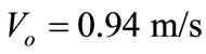 .
.
5.1.2. Discussion of Case Study 1 Results
Comparison of numerical results with measured results needs to consider several parameters such as the rate of air (Equation (24)) and the static friction. As shown by Wylie and Streeter [27], the rate of air reduces pressure wave celerity. This reduction is reflected in the numerical model by an increase in the pressure-oscillation period. This analysis was used to estimate the rate of air. Simulations were performed to find the value of the rate of air for better correspondence between measured and calculated oscillations. The rate of air is then considered to be 0.02%. The static friction  is selected from Axworthy et al. [28], who compared their numerical results to the experimental results of Adamkowski and Lewandowski [24]. The polytropic coefficient is considered as
 . After several simulations, this value, corresponding to adiabatic conditions, seemed to yield best results.
Comparison between simulated and measured results (Figure 1) shows good correlation with the frequency of oscillations. The period of frequency is slightly larger in the case without taking into account the dynamical friction component. There is a slight overestimation of pressure when the dynamical friction is not taken into account, which may reach a maximum of 3 m at the downstream end of the pipe. For pressure amplitudes, the difference between measured and simulated results increases over time. This indicates that the dissipation of the numerical model is not sufficient; in other words, the friction coefficient is underestimated. This may be due either to the static friction component or the dynamic friction component. Moreover, the increased gap between numerical results and measurements may be due to the Brunone coefficient calculation by Equations (9) and (10). Indeed the difference becomes important beyond 2.5 s, i.e. when the Reynolds number in the peak pressure falls below 6000. This shows that when the flow dissipates or becomes less turbulent, the coefficient  becomes less accurate.
5.2. Case Study 2: Closed Upstream Valve Analysis
5.2.1. Experimental Setup of the Case Study 2
The experimental tests used to examine the unsteadyflow, in case of a closed valve installed upstream just after the pump are taken from Pezzinga and Scandura [29]. These results are extracted from the paper by Prashanth Reddy et al. [6]. The tests were carried out on experimental installation composed of a zinc-plated steel pipeline (length 143.7 m, diameter 53.2 mm, thickness 3.35 mm, modulus of elasticity 2.06 × 10¹¹ N/m2, roughness 0.1 mm) fed by a centrifugal electropump. A 1 m3 pressure tank is located at the downstream end of the pipe. Closing the upstream valve generates an interesting transient flow useful for analyzing dynamic friction.
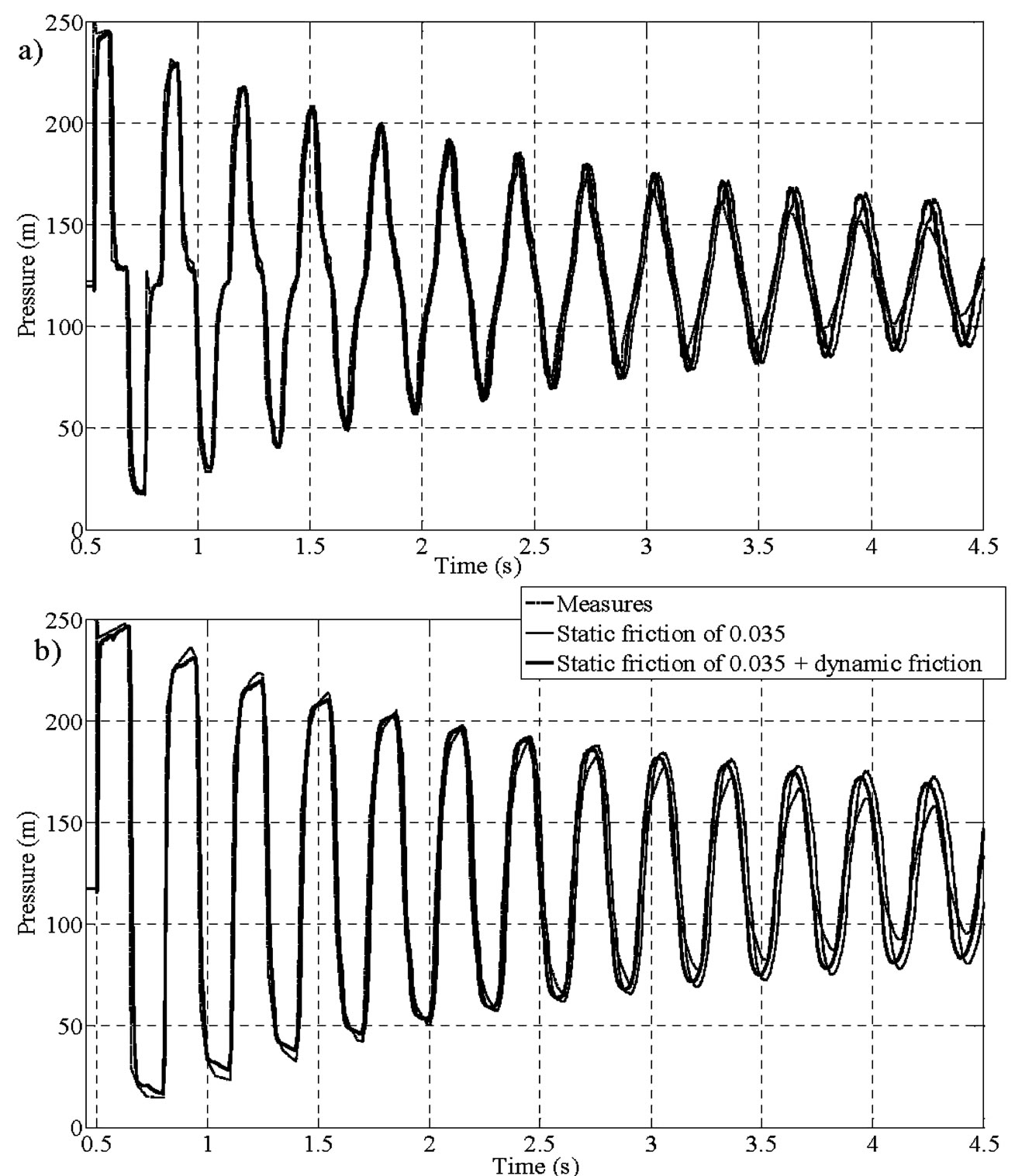
Figure 1. Comparison between calculated and measured pressure (measures reported in Adamkowski and Lewandowski [24]): a) at pipe middle; b) at pipe end.
The pressure variation is measured by pressure transducers located at the upstream valve and at the middle of the pipe. The average temperature of the water during the tests was 15˚C; the values of the kinematic viscosity  and of the elastic modulus K were assumed to be 1.14 × 10⁻⁶ m2/s and 2.14 × 10⁹ N/m2, respectively. The theoretical pressure wave celerity considered by the authors [29] is equal to 1360 m/s. As with the downstream valve in Case Study 1, a low rate of air into the water is assumed. Several simulations are performed with different rates of air to find out which allows for a better comparison between calculated and measured pressure oscillations. The initial velocity in the pipe, before closing of the valve, is
 , and the static friction component is considered equal to
 .
.
5.2.2. Discussion of Case Study 2 Results
Figure 2 shows the comparison between calculated and measured pressure values. The best superposition of oscillations is obtained with a rate of air of 0.01% and a polytropic coefficient considered equal to . The calculated frequencies of oscillations coincide perfectly with those measured at the valve and at the middle of the pipe. Consideration of the static friction component or dynamic friction component shows that they tend to dissipate energy. The inclusion of the dynamic friction
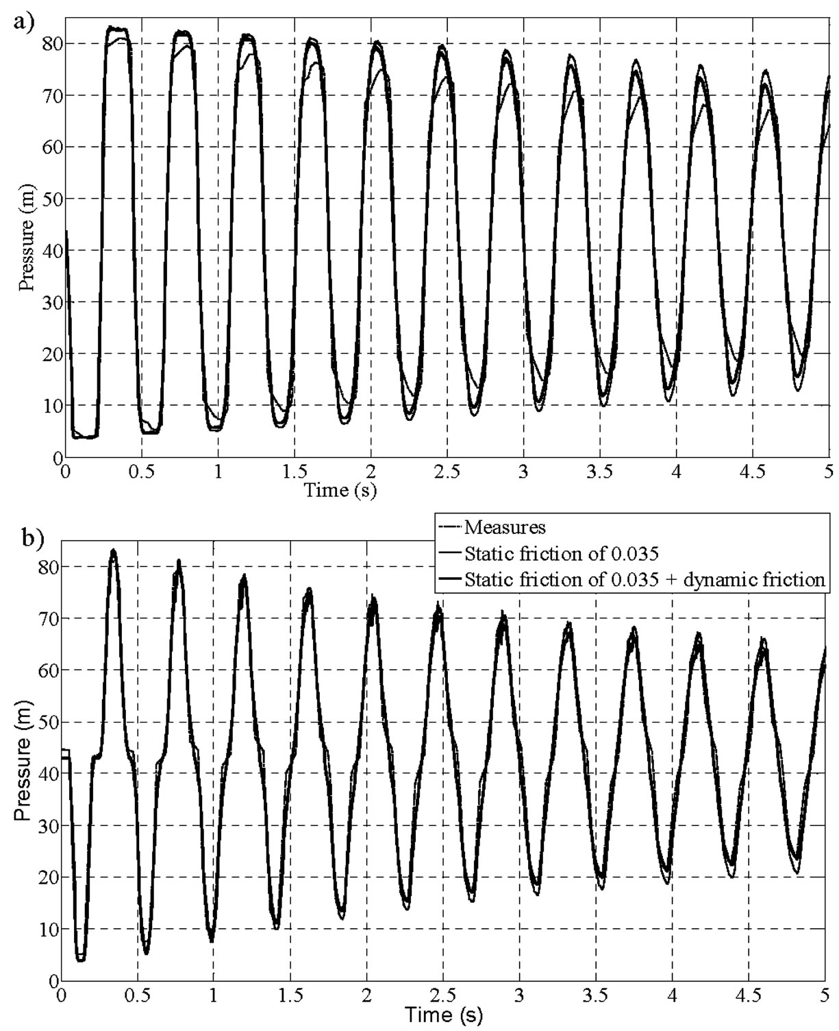
Figure 2. Comparison between calculated and measured pressure by Pezzinga and Scandura [29]: a) at the valve location; b) at the middle of the pipe.
component enables a better agreement between calculated and measured pressure values. The maximum difference obtained is 6%, and is greatest at the valve position. This difference may be due to the boundary condition calculation. The difference between measured and calculated pressure values is very low in the first pressure peaks, i.e., just after the valve closure. These pressure peaks are the most damaging to water plants. Overall, the numerical results tend to overestimate pressure values, especially at the valve position, which may be due to the choice of static friction, the initial flow condition before the valve closure, the boundary condition calculation, or the early stage of computing. Another factor that might affect the quality of results is the choice of the rate of air. The choice of the polytropic coefficient may also influence the quality of results. Experiments are rarely realized under ideal adiabatic  or isothermal
  conditions. Thus, tests with a uniform measure of the rate of air are needed to better calibrate the model.
6. Conclusions and Recommendations
This paper focuses on the resolution of unsteady friction using the Godunov approach in a finite volume method with single-equivalent two-phase flow equations. The calculated results show good agreement with experimental measurements, especially for the first pressure peaks, which are the most dangerous for pipe safety. However, dissipation is found to be lower in the calculated than in the measured results. The differences between simulated results with a dynamic friction component and those with a static friction component are more important in the case of a closed upstream valve than a closed downstream valve. It would appear that taking the dynamic friction component into account is more relevant in the case of upstream valve closure. This could be due partly to the formalization of the dynamic friction component, and in particular, the inclusion of acceleration and deceleration, as well as direction of flow. The difference could also be due to the calculation of boundary conditions, which are different in the two case studies. These results demonstrate that the proposed approach allows dynamic friction to be taken into account in finite-volume models, using the increasingly popular Godunov approach. The results also point to the possibility of considering the effect of air in order to improve the quality of simulation models. The model requires further improvements to more accurately reproduce the pressure values in cases of upstream valve closure. Searching for an adequate solution should address the determination of boundary conditions, the formalization of the dynamic friction component and the choice of the polytropic coefficient and experiments in which all parameters are adequately defined.
REFERENCES
- W. Zielke, “Frequency-Dependent Friction in Transient Pipe Flow,” Journal of Basic Engineering, Vol. 90, No. 1, 1968, pp. 109-115. http://dx.doi.org/10.1115/1.2926516
- K. Suzuki, T. Taketomi and S. Sato, “Improving Zielke’s Method of Simulating Frequency-Dependent Friction in Laminar Liquid Pipe Flow,” Journal of Fluids Engineering, Vol. 113, No. 4, 1991, pp. 569-573.
- G. Schohl, “Improved Approximate Method for Simulating Frequency-Dependent Friction in Transient Laminar Flow,” Journal of Fluids Engineering; (United States), Vol. 115, No. 3, 1993.
- A. E. Vardy and J. M. B. Brown, “Transient Turbulent Friction in Smooth Pipe Flows,” Journal of Sound and Vibration, Vol. 259, No. 5, 2003, pp. 1011-1036. http://dx.doi.org/10.1006/jsvi.2002.5160
- A. E. Vardy and J. M. B. Brown, “Transient Turbulent Friction in Fully Rough Pipe Flows,” Journal of Sound and Vibration, Vol. 270, No. 1-2, 2004, pp. 233-257. http://dx.doi.org/10.1016/S0022-460X(03)00492-9
- H. P. Reddy, W. F. Silva-Araya and M. H. Chaudhry, “Estimation of Decay Coefficients for Unsteady Friction for Instantaneous, Acceleration-Based Models,” Journal of Hydraulic Engineering, Vol. 138, No. 3, 2012, pp. 260- 271. http://dx.doi.org/10.1061/(ASCE)HY.1943-7900.0000508
- J. Vítkovský, M. Stephens, A. Bergant, A. Simpson and M. Lambert, “Numerical Error in Weighting FunctionBased Unsteady Friction Models for Pipe Transients,” Journal of Hydraulic Engineering, Vol. 132, No. 7, 2006, pp. 709-721. http://dx.doi.org/10.1061/(ASCE)0733-9429(2006)132:7(709)
- B. Brunone, B. W. Karney, M. Mecarelli and M. Ferrante, “Velocity Profiles and Unsteady Pipe Friction in Transient Flow,” Journal of Water Resources Planning and Management, Vol. 126, No. 4, 2000, pp. 236-244. http://dx.doi.org/10.1061/(ASCE)0733-9496(2000)126:4(236)
- B. Brunone, U. M. Golia and M. Greco, “Effects of TwoDimensionality on Pipe Transients Modeling,” Journal of Hydraulic Engineering, Vol. 121, No. 12, 1995, pp. 906- 912. http://dx.doi.org/10.1061/(ASCE)0733-9429(1995)121:12(906)
- A. Bergant, A. R. Simpson and J. Vitkovsky, “Developments in Unsteady Pipe Flow Friction Modelling,” Journal of Hydraulic Research/De Researches Hydrauliques, Vol. 39, No. 3, 2001, pp. 249-257.
- J. P. Vítkovský, A. Bergant, A. R. Simpson and M. F. Lambert, “Systematic Evaluation of One-Dimensional Unsteady Friction Models in Simple Pipelines,” Journal of Hydraulic Engineering, Vol. 132, No. 7, 2006, p. 696. http://dx.doi.org/10.1061/(ASCE)0733-9429(2006)132:7(696)
- G. Pezzinga, “Quasi-2D Model for Unsteady Flow in Pipe Networks,” Journal of Hydraulic Engineering, Vol. 125, No. 7, 1999, pp. 676-685. http://dx.doi.org/10.1061/(ASCE)0733-9429(1999)125:7(676)
- G. Pezzinga, “Evaluation of Unsteady Flow Resistances by Quasi-2D or 1D Models,” Journal of Hydraulic Engineering, Vol. 126, No. 10, 2000, pp. 778-785. http://dx.doi.org/10.1061/(ASCE)0733-9429(2000)126:10(778)
- B. Brunone, U. M. Golia and M. Greco, “Modeling of Fast Transients by Numerical Methods,” Proceedings of International Conference on Hydraulic Transients with Water Column Separation, IAHR-Group, Madrid, 1991, pp. 273-280.
- M. Bughazem and A. Anderson, “Problems with Simple Models for Damping in Unsteady Flow,” Proceedings of International Conference on Pressure Surges and Fluid Transients, BHR Group, Harrogate, 1996, pp. 537-548.
- M. Bughazem and A. Anderson, “Investigation of an Unsteady Friction Model for Waterhammer and Column Separation,” 8th International Conference on Pressure Surges, BHR Group, The Hague, 2000, pp. 483-498.
- E. B. Wylie, “Frictional Effects in Unsteady Turbulent Pipe Flows,” Applied Mechanics Reviews, Vol. 50, No. 11S, 1997, pp. S241-S244. http://dx.doi.org/10.1115/1.3101843
- M. H. Chaudhry, “Open-Channel Flow,” 2nd Edition, Springer, 2008, p. 523.
- E. F. Toro, “Shock Capturing Methods for Free Surface Shallow Flows,” John Wiley and Sons, 2001, p. 326.
- V. Guinot, “Godunov-Type Schemes: An Introduction for Engineers,” Elsevier, Amsterdam, 2003.
- A. S. León, M. S. Ghidaoui, A. R. Schmidt and M. H. Garcia, “A Robust Two-Equation Model for Transient-Mixed Flows,” Journal of Hydraulic Research, Vol. 48, No. 1, 2010, pp. 44-56. http://dx.doi.org/10.1080/00221680903565911
- J. G. Vasconcelos and S. J. Wright, “Comparison between the Two-Component Pressure Approach and Current Transient Flow Solvers,” Journal of Hydraulic Research, Vol. 45, No. 2, 2007, pp. 178-187. http://dx.doi.org/10.1080/00221686.2007.9521758
- B. F. Sanders and S. F. Bradford, “Network Implementation of the Two-Component Pressure Approach for Transient Flow in Storm Sewers,” Journal of Hydraulic Engineering, Vol. 137, No. 2, 2011, p. 15.
- A. Adamkowski and M. Lewandowski, “Experimental Examination of Unsteady Friction Models for Transient Pipe Flow Simulation,” Journal of Fluids Engineering, Vol. 128, No. 6, 2006, pp. 1351-1363. http://dx.doi.org/10.1115/1.2354521
- A. Bergant, A. R. Simpson, U. O. A. D. O. Civil and E. Engineering, “Water Hammer and Column Separation Measurements in an Experimental Apparatus,” Department of Civil and Environmental Engineering, University of Adelaide, 1995.
- V. Guinot, “Numerical Simulation of Two-Phase Flow in Pipes Using Godunov Method,” International Journal for Numerical Methods in Engineering, Vol. 50, No. 5, 2001, pp. 1169-1189. http://dx.doi.org/10.1002/1097-0207(20010220)50:5<1169::AID-NME71>3.0.CO;2-#
- B. E. Wylie and V. L. Streeter, “Fluid Transients in Systems. Prentice Hall, Englewood Cliffs, NJ 07632, USA,” 1993.
- D. H. Axworthy, M. S. Ghidaoui and D. A. McInnis, “Extended Thermodynamics Derivation of Energy Dissipation in Unsteady Pipe Flow,” Journal of Hydraulic Engineering, Vol. 126, No. 4, 2000, pp. 276-287. http://dx.doi.org/10.1061/(ASCE)0733-9429(2000)126:4(276)
- G. Pezzinga and P. Scandura, “Unsteady Flow in Installations with Polymeric Additional Pipe,” Journal of Hydraulic Engineering, Vol. 121, No. 11, 1995, pp. 802-811. http://dx.doi.org/10.1061/(ASCE)0733-9429(1995)121:11(802)