Journal of Water Resource and Protection
Vol. 5 No. 3A (2013) , Article ID: 29238 , 14 pages DOI:10.4236/jwarp.2013.53A037
Nutrient Input and CO2 Flux of a Tropical Coastal Fluvial System with High Population Density in the Northeast Region of Brazil
1Departamento de Oceanografia, Centro de Estudos e Ensaios em Riscos e Modelagem Ambiental, Universidade Federal de Pernambuco, Recife, Brazil
2Laboratoire d’Océanographie et du Climat: Expérimentation et Approches Numériques, Université Pierre et Marie Curie. 4, Paris, France
Email: *moa@ufpe.br
Received December 29, 2012; revised January 31, 2013; accepted February 10, 2013
Keywords: Tropical River; Nutrient Load; CO2 Flux; Anthropogenic Pollution; Freshwater Ecosystem Impact
ABSTRACT
The carbon dioxide flux through the air-water interface of coastal freshwater ecosystems must be quantified to understand the regional balances of carbon and its transport through coastal and estuarine regions. The variations in air-sea CO2 fluxes in nearshore ecosystems can be caused by the variable influence of rivers. In the present study, the amount of carbon emitted from a tropical coastal river was estimated using climatological and biogeochemical measurements (2002-2010) obtained from the basin of the Capibaribe River, which is located in the most populous and industrialized area of the northeast region of Brazil. The results showed a mean CO2 flux of +225 mmol·m−2·d−1, mainly from organic material from the untreated domestic and industrial wastewaters that are released into the river. This organic material increased the dissolved CO2 concentration in the river waters, leading to a partial pressure of CO2 in the aquatic environment that reached 31,000 μatm. The months of April, February and December (the dry period) showed the largest monthly means for the variables associated with the carbonate system ( , DIC, CO2(aq),
  , TA, temperature and pH). This status reflects the state of permanent pollution in the basin of the Capibaribe River, due, in particular, to the discharge of untreated domestic wastewater, which results in the continuous mineralization of organic material. This mineralization significantly increases the dissolved CO2 content in the estuarine and coastal waters, which is later released to the atmosphere.
1. Introduction
Rivers and estuaries play an important role in the transport and transformation of carbon from the continent to the adjacent coastal zone and typically act as liquid sources of CO2 to the atmosphere [1-3]. Although approximately 60% of the global freshwater inputs and 80% of the total organic carbon occur at tropical and subtropical latitudes [4,5], the number of works that have quantified the air-water exchanges of CO2 in tropical estuaries and rivers is still extremely limited [6].
Recent studies estimate that rivers supply 0.8 - 1.33 PgC to the oceans worldwide, of which ~0.53 PgC is transported from tropical rivers (30˚N - 30˚S) to adjacent estuarine systems [7]. Nearshore coastal systems, such as estuaries, saltmarsh waters, mangroves mangrove swamps, coral reefs, and coastal upwelling systems, generally act as sources of CO2, and a preliminary analysis suggested that the overall emission of CO2 from these systems could be as high as 0.40 PgC·yr−1, thus balancing the CO2 sink associated with marginal seas [1,6]. A recent study [8] evaluated the exchange of CO2 between inner estuaries and the atmosphere based on a compilation of 62 systems. The computed emission of +0.27 ± 0.23 PgC·yr−1 given by this study is lower than previous estimates, which range between +0.36 and +0.60 PgC·yr−1 [1,9,10]. However, all recent studies have shown higher values than the first reported estimations (0.1 PgC·yr−1) [11].
Most studies prior to 2005 covered estuaries that were located largely in the mid-to-high latitudes (mostly in Europe). Estuaries at the lower latitudes received less attention, although the total surface area of the low-latitude estuaries is larger than that of the estuaries in midand high-latitude systems [1]. According to [6], the average CO2 effluxes from low-latitude (0˚ - 30˚) and mid-latitude (30˚ - 60˚) estuaries are 17 and 46 mol CO2 m−2·yr−1, respectively. A recent study [12] reported an efflux of 13 mol CO2 m−2·yr−1 for a tropical estuary (the Piauí estuary, Brazil, latitude 10˚S). As indicated by [6], the current calculation is based on a very limited data set from subtropical and tropical regions. Estimates of the variability in air-sea CO2 fluxes on seasonal and interannual time scales in tropical estuaries are necessary to help constrain the net partitioning of CO2 between the atmosphere, oceans and terrestrial biosphere.
In Brazil, and particularly in the northeastern region of the country, very little is known about the seasonal and interannual variability of the CO2 flux at the air-water interface in rivers, and even less is known about its longterm evolution given the increase of atmospheric CO2.
According to [13,14], the interannual variations of air-sea CO2 fluxes in nearshore ecosystems can be caused by a variable river influence. The chemical processes that involve fluvial carbon are intimately associated with the organic and inorganic forms of carbon and their atmospheric and lithological origins [15]. Thus, quantifying the CO2 flux through the air-water interface of freshwater ecosystems is necessary to understand regional carbon balances and the relative contributions of these systems to the planetary increase of atmospheric CO2.
The objective of the present study was to characterize and quantify the seasonal and interannual variability of CO2 fluxes and the variables associated with the carbonate system in a tropical river that is located in a highpopulation-density urban area. The Capibaribe River was selected because it is highly representative based on the large number of tropical coastal systems in Brazil and throughout the world that experience high anthropogenic pressure. The waters of the Capibaribe River are subjected to an intense eutrophication process [16], resulting mainly from its proximity to the Metropolitan Region of Recife (from now on referred to as RMR—Região Metropolitana do Recife), the most populous and Industrialized area in northeastern Brazil
2. Methodology
2.1. Study Area
The hydrographic basin of the Capibaribe River covers 7557.42 km2 and is located in the coastal region of the State of Pernambuco, Brazil (Figure 1). Lithologically, the Capibaribe River basin is composed of 90% crystalline basement and 10% sedimentary basin. In the lower Capibaribe River, near the MRR, the Tertiary-aged Barreiras formation is represented by disperse sedimentary deposits that indistinctly cover the crystalline basement and the sedimentary basin. Natural vegetation covers 56.3% of the total drainage area of the Capibaribe River, with 38.8% represented by agricultural areas, 3.14% attributed to urban areas and 0.45% occupied by the continental water body [17]. Given its wide geographical coverage, the Capibaribe basin exhibits a complex environment that is characterized by climatic contrasts in the terrain, soils and vegetation cover and marked socioeconomic gradients. From its headwaters, located 240 km from the coastline, to its mouth in the MRR, the river crosses 42 municipalities, of which 15 are completely comprised within the basin, and 26 have their administrative center in this basin [17]. The total population of the basin is 1,450,000 inhabitants [18,19], for a mean population density in the basin of 190 inhabitants km−2, with the highest concentration in the MRR (1000 inhabitants km−2).
Various activities occur in the basin, and the main activities include the production of food, non-metallic minerals, textiles, metallurgy, chemicals, pharmaceutical products, veterinary products, sugars/ethanol, leathers, plastic materials, drinks, transport materials and wood. The residual organic load that effectively reaches the body of water is estimated at 32.4 t biochemical oxygen demand (BOD) day−1, of which 95.7% is of domestic origin and 4.3% is of industrial origin [19]. Furthermore, according to [17], the residual organic load can reach values of up to 28 t BOD day−1 at collection station CB-72/CPRH (Figure 1).
2.2. Climatology and Fluvial Discharge
The Capibaribe River basin exhibits a high spatial variability in precipitation, with mean annual values between 600 mm and 2400 mm (mean = 1133 mm from 1990 to 2010), with an increase in precipitation closer to the coast. This spatial variability reflects the influence of the two main atmospheric systems that affect the eastern edge of the northeast region of Brazil, the Intertropical Convergence Zone and the Atmospheric Easterly Waves [17,20]. Potential evapotranspiration is approximately 1700 mm, with a decrease near the coast, where the value falls to 1500 mm.
The mean annual temperature in the Capibaribe River basin varies between 20.4˚C and 26.1˚C, while the maximum temperature oscillates between 25.5˚C and 29.9˚C. Throughout the year, the temperatures in the region display a variability that can be represented by two seasons: a period with lower monthly means between April and September and the period from October to March, during which the mean temperature values increase. The winds vary between 2 m·s−1 and 5 m·s−1, with the months of August, September and December displaying the highest monthly wind speeds [21]. The mean fluvial discharge in the São Lourenço da Mata station (Figure 1) is 13.74 m3·s−1, resulting in a specific flow
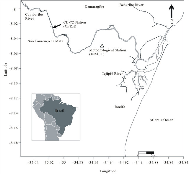
Figure 1. Capibaribe River Basin with the location of sampling station CB-72 (CPRH—Pernambuco State Environmental Agency) and the Várzea Meteorological Station (INMET—Brazilian National Institute of Meteorology).
rate of 9.79 L·s−1·km−2 [17].
In the present study, the climatological and fluvial discharge variables were analyzed using a historical time series of 20 years (1990-2010), with a special focus on the period that included biogeochemical and river water quality data (2002-2010). These last data were sampled and analyzed bimonthly from 2002-2010 at Station CB-72 (Figure 1), which is under the responsibility of the State Agency of the Environment and Water Resources (Agência Estadual de Meio Ambiente e Recursos Hídricos—CPRH) [19]. As will be discussed later, the statistical significance between these two series of physical data (climatology and river flow) was assessed to detect trends and verify the climatological representativeness of the performed analyses for 2002 to 2010, for which river water quality data were available, making the simultaneous use of physical and biogeochemical data possible.
The fluvial discharge values were obtained from the database of the National Water Agency of Brazil (Agência Nacional de Águas—ANA) [22], while the data on air temperature and pluviometric precipitation were obtained from the Brazilian National Institute of Meteorology (Instituto Nacional de Meteorologia—INMET) [21].
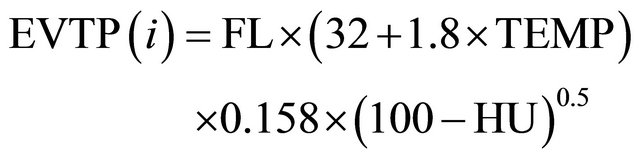
The historical series of evaporation data was obtained from the Department of Water Resources (Secretaria de Recursos Hídricos—SRH) [17], and the evapotranspiration rate was determined as follows using the Hargreaves method [23] and data on the latitude, air temperature and relative humidity:
 (1)
(1)
where EVTP (i) = Hargreaves’ potential evapotranspiration for month “i” (mm); FL = factor latitude (calculated as in [23]); TEMP = monthly mean temperature (˚C); and HU = mean monthly relative humidity (%).
2.3. Air-Water CO2 Flux
The air-water CO2 flux was determined based on bimonthly measurements (2002 to 2010) of pH, temperature, salinity and alkalinity that were obtained at station CB-72 of the CPRH in combination with climatological data (precipitation, wind intensity and atmospheric pressure) from the Meteorological Station of INMET (Figure 1).
The dissolution constants for carbonic acid that were used in the calculations were obtained from [24] for salinities of 0.1 - 50 and temperatures of 1˚C - 50˚C. The CO2 solubility coefficient was calculated using the equations in [25], and the dissociation constants of sulfate [26] and borate [27] were calculated as follows:
 (2)
(2)
where FCO2 = CO2 flux at the air-water interface (mmol·m−2·d−1); k (CO2) = gas-transfer rate (m·s−1); KH = CO2 solubility, calculated according to [25] (m·L−1 atm−1); and  = difference between the partial pressure of CO2 on the water surface (pCO2(aq)) and in the atmosphere (pCO2(air)) (μatm).
A positive value of  indicates a liquid flux of water to the atmosphere. The partial pressure of atmospheric CO2 was obtained through the following equation:
 (3)
(3)
where Patm = barometric pressure, obtained from the local meteorological data (atm); xCO2 = mole fraction of atmospheric CO2, obtained from NOAA (http://esrl.noaa. gov) (ppm); and pH2O = water vapor pressure (μatm), obtained from [28].
The water vapor pressure was determined using the following equation:
 (4)
(4)
where sst = the sea surface temperature of the body of water (˚K) and S = the salinity of the body of water.
The gas-transfer rate was calculated using the equation from [29] as follows:
 (5)
(5)
where u10 is the wind speed at 10 m from the surface of the body of water (m·s−1) and Sc is the Schmidt number.
The results obtained from Equations (2)-(5), combined with the results from the analyses of the mineral nutrients [19], were used as input data for the CO2 calcÒ software [30]. This software uses the equations of the carbonate system to obtain pCO2 in the water,  , CO2 aqueous,
  , dissolved inorganic carbon (DIC) and other parameters derived from the carbonate system.
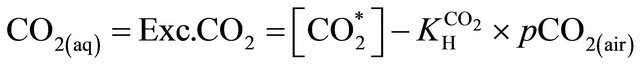
The excess of CO2 (CO2(aq)) (μmol·kg−1) is defined as the amount of DIC that is transferred as CO2 to the atmosphere after attaining air-water equilibrium. The excess of CO2 was calculated according to the equation from [31], as follows:
 (6)
(6)
where  is the concentration of total free CO2 in
μmol·kg−1 (i.e.,
 in water)
and  is the solubility coefficient of CO2.
The apparent oxygen utilization (AOU, μmol·kg−1) was determined based on the equation in [32]:
 (7)
(7)
with the dissolved oxygen saturation (%O2) calculated according to the following equation:
 (8)
(8)
where [O2]eq = the dissolved oxygen (DO) concentration at equilibrium with the atmosphere, calculated based on [33] and the local air pressure (μmol·kg−1); [%O2] = DO saturation (%); O2 = in situ DO concentration (μmol·kg−1); and  = solubility of oxygen as a function of temperature and salinity (μmol·kg−1).
The statistical analyses (t-test, trend, PCA and descriptive statistics) were performed using XLSTAT® 2010 software. The non-parametric Mann-Kendall test was selected, which is widely utilized to detect monotonic trends in data series, without the need to specify whether these trends are linear.
3. Results
3.1. Climatology and Fluvial Discharge
The air temperature, pluviometric precipitation and evaporation did not show significant differences between the historical period (1990-2010) and the study period (2002-2010) (t-test; α = 0.05) (Figures 2(a)-(c)). The annual water balance was positive, with a seasonal variability characterized by 6 months of positive water balance (March to August) and 6 months of negative water balance (September to February). According to the Mann-Kendall trend test (α = 0.05), the observed data on precipitation, temperature and humidity did not show significant increasing or decreasing trends for these variables.
Fluvial discharges did not show significant differences between the historical period and the study period (t-test; α = 0.05) (Figure 2(e)). The mean flow rate for the study

Figure 2. Seasonal variability in the Capibaribe River basin, Brazil, calculated based on the historical time series 1990-2010 (black bars) and the period 2002-2010 (gray bars): (a) Precipitation; (b) Evaporation; (c) Air temperature; (d) Wind speed and (e) Fluvial discharge. Wed period = March-August, dry period = September-February.
period was 11.8 m3·s−1, which was very similar to the value of 13.7 m3·s−1 obtained for the historical period (1990-2010) [17]. Based on the Mann-Kendall test (α = 0.05), there was no significant trend (increasing or decreasing) in the flow rate data from 1990-2010.
The wind intensities show significant differences between the historical period and the study period (t-test; α = 0.05). The mean annual value recorded in the period from 2002-2010 of 2.2 m·s−1 was lower than the historical mean value of 2.6 m·s−1. All of the monthly wind intensities were lower than those recorded historically in the region (Figure 2(d)). Based on the Mann-Kendall test (α = 0.05; p < 0.0001), there was a positive (growing) trend among the historical wind data (1990-2010).
3.2. Water Temperature, Salinity, Organic Load (BOD) and Dissolved Oxygen (DO%)
Water temperature and salinity did not show significant trends according to the Mann-Kendall test (α = 0.05), indicating the repetitive cyclical nature of these state variables in the study period. The coefficient of variation for both state variables was minimal (0.1 and 0.4, respecttively). According to the t-test (α = 0.05; p < 0.002), the mean seasonal water temperatures (March-August x September-February) showed significant differences between the wet and dry periods of the year. The amplitude of the means was 1.5˚C (wet = 27.1˚C and dry = 28.6˚C).
The mean salinity value was 0.3 ± 0.01 units, with maximum values in February (dry period) and minimum values in June (wet period), indicating that salinity follows the climatic seasonal cycle. The salinity in this section of the river was classified as freshwater (94% of the values were <0.5).
The mean BOD concentration was 4.4 ± 3 mg·l−1 from 2002-2010. When this concentration was associated with fluvial discharge, a mean input of 53.1 t BOD·d−1 in the Capibaribe River was obtained, which represents 63.8% more than the residual pollution load that was reported by the CPRH for 2010 (32.4 t BOD·d−1). The data observed do not show significant differences (α = 0.05; p < 0.9) in the mean concentrations of organic load between the dry and wet periods. The data series for the BOD concentration of the period 2002-2010 showed a maximum value of 16.7 mg·l−1 and a minimum of 0.5 mg·l−1 (Figure 3(b)). Values above 5 mg·l−1 are above the legal limit recommended by the Brazilian legislation for this type of water source [34]. According to the Mann-Kendall test, there is a positive trend in the BOD data (α = 0.05; p < 0.025), indicating a gradual increase in the levels of biodegradable organic material during the study period.
The dissolved oxygen saturation (DO%) showed a mean value of 44% ± 20%, with a mean DO concentration of (95 ± 70 μmol·kg−1) (3.04 ± 2 mg·l−1) during 2002- 2010. The highest monthly mean was recorded in October (during the dry period), while the lowest value was observed in April (during the wet period) (Figure 3(b)).
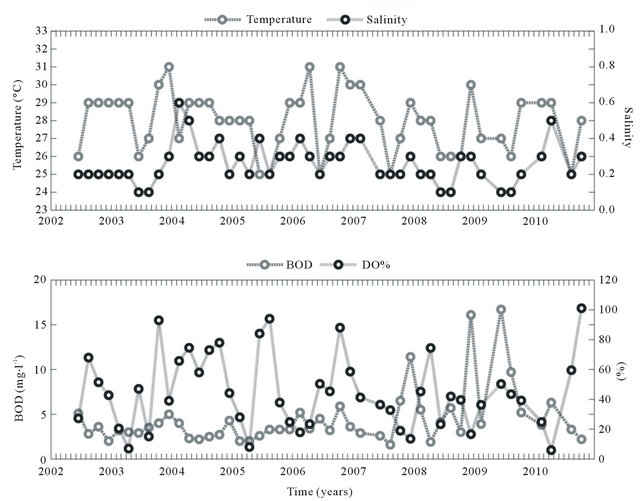
Figure 3. Water temperature, salinity, biochemical oxygen demand (BOD) and saturation of dissolved oxygen (DO%) in the Capibaribe River, Brazil.
Values less than 5 mg·l−1 are below the limit recommended by the Brazilian legislation [34]. During the study period, 78% of the samples exhibited concentrations below this limit (5 mg·l−1).
According to the t-test (α = 0.05; p < 0.25), the data did not show significant differences between the dry and rainy periods. Based on the Mann-Kendall test, the DO% did not show significant alteration trends (α = 0.05) from 2002-1010.
3.3. Dissolved Inorganic Carbon (DIC), Total Alkalinity (TA), pH and Mineral Nutrients ( and
and )
)
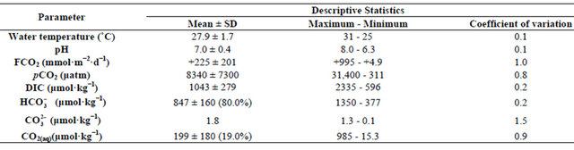
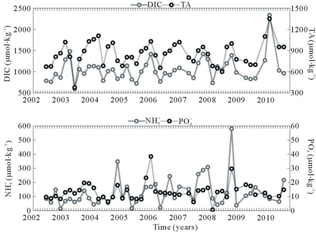
The DIC concentration during 2002-2010 showed a smaller variation than the other parameters associated with the carbonate system (596 to 2,235 μmol·kg−1; coefficient of variation = 0.2) (Figure 4(a)). The data did not show significant differences (α = 0.05; p < 0.2) between the dry and rainy periods. Based on the Mann-Kendall test (α = 0.05), the DIC did not show a positive trend during 2002-2010, suggesting a continuous input of carbon inorganic species throughout the years. The mean distribution of the compounds that comprise DIC was as follows:  = 80.8%;
  = 0.2% and CO2(aq) = 19% (Table 1). Of these compounds,
  and CO2(aq) displayed a higher coefficient of variation and thus influence the variation of the DIC concentration in the Capibaribe River.
The TA showed a mean value of 851 ± 160 μmol·kg−1 during 2002-2010 (Figure 4(a)). The estimated values showed significant differences between the dry and wet periods (α = 0.05; p < 0.004), with a higher mean during the dry period (920 μmol·kg−1). The variance was 377 - 1350 μmol·kg−1 (coefficient of variation = 0.2). Based on the Mann-Kendall test (α = 0.05), the TA did not show a positive trend during 2002-2010, indicating that the concentrations recorded in this period were constant. The highest monthly mean was observed in February (942 μmol·kg−1), while the lowest monthly mean TA occurred in June (674 μmol·kg−1).
The waters of the Capibaribe River show high concentrations of mineral nutrients that serve as important fertilizers in the adjacent estuarine and coastal waters [16]. The  and
and  concentrations measured during
Table 1. Variables associated with the carbonate system in the Capibaribe River, Brazil, during 2002-2010. Mean values in parentheses represent the proportion (%) of the total DIC.
 (a)
(a) (b)
(b)
Figure 4. (a) Concentration of dissolved inorganic carbon (DIC), total alkalinity (TA), ammonia ( ) and orthophosphate (
 ) in the Capibaribe River, Brazil; (b) pH and concentration of bicarbonate (
 ) in the Capibaribe River, Brazil.
2002-2010 were above the corresponding limits recommended by the legislation [34]. The period from October to February (the dry period) systematically showed the highest concentrations of dissolved nutrients, reaching 38 μmol·kg−1 for  and 580 μmol·kg−1 for
  (Figure 4(a)).
The pH values measured in the Capibaribe River did not show significant differences (α = 0.05; p < 0.9) between the wet period and the dry period. The mean of the series was 7.0 ± 0.4; however, low values were observed in both climatic periods (Figure 4(b) and Table 1).
The  concentrations showed significant differences (α = 0.05; p < 0.04) between the wet and the dry period (Figure 4(b) and Table 1).
3.4. Partial Pressure of CO2 in the Water (pCO2(aq)) and CO2 Flux (FCO2)
The partial pressure of carbon dioxide in the Capibaribe River was highly variable throughout the study period (coefficient of variation = 0.8), ranging between 311 and 31,400 μatm, with a mean value of 8340 μatm (Figure 5(a) and Table 1). The pCO2(aq) values did not show significant differences between the dry and rainy periods (α
= 0.05; p < 0.6). The highest monthly mean was recorded in April (17,440 μatm) (Table 1). Based on the MannKendall test (α = 0.05), the partial pressure of CO2 did not show a significant positive or negative trend during 2001-2010, indicating that the concentrations were consistent throughout the analyzed temporal series.
The progression of the CO2 flux (FCO2) in the Capibaribe River was always positive during the study period, with a mean value of +225 mmol·m−2·d−1, indicating a continuous release of CO2 into the atmosphere (Figure 5(b)). The highest value calculated in the period was +995 mmol·m−2·d−1 (April 2010), and the lowest flux was +4.9 mmol·m−2·d−1 (August 2005), thus supporting the high coefficient of variation (Figure 5(b) and Table 1). Similarly to the water partial pressure, the FCO2 values did not show significant differences between the dry and rainy periods (α = 0.05; p < 0.5). The highest monthly mean was also recorded in April (+426 mmol·m−2·d−1), while the lowest monthly mean value was observed in August (+119 mmol·m−2·d−1). Based on the Mann-Kendall test (α = 0.05), the CO2 fluxes did not show trends (positive or negative) during 2001-2010, indicating an almost continuous release to the atmosphere over the period analyzed.
 (a)
(a)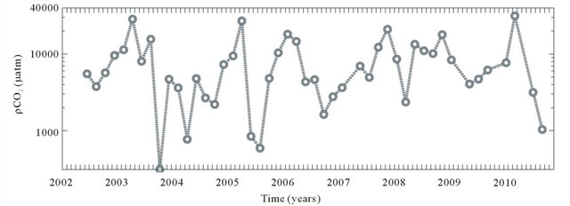 (b)
(b)
Figure 5. CO2 partial pressure in water (pCO2(aq)) and CO2 water-air flux (FCO2) in the Capibaribe River, Brazil.
4. Discussion
The processes that partition dissolved CO2, pCO2(aq) and DIC in fluvial environments are complex and influenced by a combination of sources and natural processes, such as the types of rock and soil in the hydrographic basin, water-atmosphere interaction sand oxidation/reduction reactions of anthropogenic inputs [15]. Based on the results presented in the previous section, an analysis of the possible agents that influence the biogeochemistry and the carbon flux in the Capibaribe River, a typical tropical coastal system that is subjected to intense anthropogenic action in the northeast region of Brazil, will be presented next. The findings for the Capibaribe River reflect an important state of pollution in the drainage basin; this pollution is mainly due to the discharge of untreated domestic wastewater into the water. The estimated population density for 2010 in the city of Recife was 7000 inhabitants km−2, and the mean density in the drainage basin reaches 191 inhabitants km−2 [18], resulting in a significant input of organic load that is released directly into the river [19].
When analyzing whether the type of rock/soil influenced the water CO2 content, no correlation between fluvial discharge and pCO2(aq) was observed (r2 = 0.01; p < 0.0001) (Figure 6(a)), suggesting that the transport processes via fluvial runoff are not the main factors that are responsible for the high concentrations of dissolved CO2 found in the Capibaribe River. Authors such as [35] have shown that the lack of correlation between these two variables is characteristic of basins that are located in populous industrialized areas. For example, in the Zenne River (urban river in Brussels, Belgium), periods of high fluvial discharge were not correlated with high pCO2(aq) values [36].
Based on Figure 6(b) and Table 2, the BOD exhibited a low correlation with pCO2(aq) (r2 = 0.04); however, DO% showed a strong negative correlation with pCO2 (r2 = 0.86; p < 0.0001; Figure 6(b)), indicating that the loads of domestic and industrial wastewaters increased during this period (2002-2010), thus increasing the organic matter decomposition and decreasing the pH (pH vs. DO%; r2 = 0.70; p < 0.0001; Figure 6(d)). Additionally, the AOU was positively correlated with the excess of CO2(aq) (r2 = 0.41; p < 0.0001; Figure 6(e)). This result indicates that the organic load that enters the Capibaribe River has a significant impact on the microbial processes that are associated with the carbon and nitrogen cycles. The nutrients enrich the water and can lead to an excessive production of algal biomass and, consequently, eutrophication. Thus, planktonic metabolism and the organic matter associated with domestic and industrial wastewaters can consume the dissolved oxygen in the water [16,37].
Nitrogen and phosphate compounds showed concentrations that are typical of bodies of water that are affected by urban inputs. The mean DIN (dissolved inorganic nitrogen) concentration was 144 μmol·kg−1, while the ammonia concentration was 134 μmol·kg−1 (~90% of the DIN value). Simultaneously, the mean DIP (dissolved inorganic phosphate) concentration was 13.2 μmol·kg−1. The DIN/DIP ratio was therefore 11:1, which is very similar to the ratio of 12:1 found by [38] for domestic and industrial waste waters; these compounds serve as a nutrient source for the microbial activity in many rivers [35]. High values of ammonium  and other nitrogen compounds (
 and
and ) in rivers and the processes associated with them, such as ammonification, nitrification and denitrification, have a strong and rapid effect on alkalinity. Under oxic conditions, ammonification produces
 , leading to
 . Underanoxic conditions, ammonification produces
 , and denitrification consumes
 . However, under both conditions, the changes in
  and
and  affect the TA [39]. Thus, despite the high TA values observed in the Capibaribe River (mean = 851 ± 160 μmol·kg−1), the analysis did not show a strong correlation between alkalinity and DO%,
  or pCO2(aq) (see Figure 7 and Table 2).
According to [35], under conditions of high CO2(aq) values, which result from bacterial respiration, carbonic acid is produced and decreases the river water pH. If the characteristics of the body of water are such that the CO2 concentration in the aqueous media are close to equilibrium with atmospheric CO2, strong correlations between alkalinity, pCO2(aq) and pH would be expected. However, the complex set of processes that lead to the production or consumption of CO2(aq) and the production or removal of carbonic acid ( ) prevent the establishment of a correlation between alkalinity, pH and pCO2(aq) [35,40]. These high alkalinity values may, therefore, be associated with the high values of
  found in the Capibaribe River, which represent 81% of the total DIC, while CO2(aq) represents 19%, and the remainder (~0.2%) was associated with
 . These values are in accordance with the values recorded for highly polluted rivers, including both tropical rivers, such as the Tietê [15] and Piracicaba [41] rivers of Brazil, and temperate rivers, namely the Zenne, Dijle and Scheldt-Belgium rivers [36]. Based on [15], the processes that are involved in the mineralization of fluvial organic matter are mainly anaerobic, with are also associated with sulfate oxidation. During sulfate oxidation,
  is primarily formed and, CO2(aq) can be produced via methanogenesis after the reoxidation of these compounds.
The DIC concentrations in the Capibaribe River (mean = 1043 μmol·kg−1) were higher than those reported by [7] for tropical rivers (645 μmol·kg−1). According to this
 (a)
(a) (b)
(b)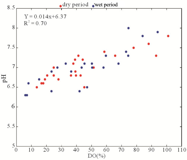 (c)
(c)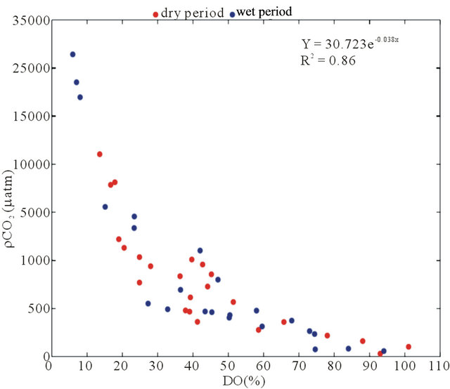 (d)
(d)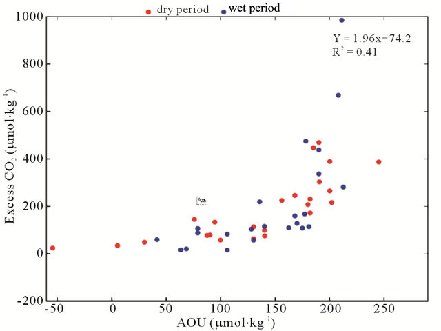 (e)
(e)
Figure 6. Correlations between the riverand carbonate system-linked variables in the 2002-2010 data series in the Capibaribe River (CB-72/CPRH). (a) pCO2 vs. fluvial discharge; (b) pCO2 vs. BOD; (c) pCO2 vs. DO%; (d) pH vs. DO% and (e) CO2 excess vs. AOU.
Table 2. Factor loadings of principal component analysis performed with the variables analyzed for the Capibaribe River, Brazil, during 2002-2010.
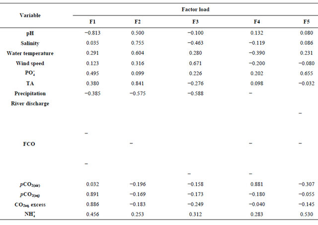

Figure 7. Principal component analysis of the variables that were investigated in the 2002-2010 period in the Capibaribe River, Brazil.
author, the dissolved organic carbon (DOC) concentrations for tropical rivers vary around 448 μmol·kg−1 and are directly associated with the organic discharges from domestic and industrial sources [42]. Following the equation proposed by [4] (DOC = 0.65 × ), a DOC concentration of 550 μmol·kg−1 was determined for the Capibaribe River. This value is 1.2 times the global mean for tropical rivers estimated by [7] and thus reinforces the high concentrations of carbonate system compounds that are associated with anthropogenic actions.
The principal component analysis (PCA) performed with the set of studied variables is shown in Figure 7 and detailed in Table 2. The PCA showed an association between the months of April, February and December with pCO2(aq), FCO2 and the variables associated with the carbonate system (DIC, TA,  ,
,  , CO2(aq)). Precipitation in the basin and the fluvial discharge in the Capibaribe River were associated with June, while the DO% was associated with August. The wind intensity and water temperature were both associated with December.
During the dry months (December and February), the mean water temperature was 1.5˚C higher when compared with the mean for the months of the wet period. During the dry period, biological activity, which is critical for the production and consumption of CO2(aq) in the rivers, is strongly influenced by physical factors such as temperature, light and fluvial discharge, and this activity can vary on a scale of minutes, days or seasonally [35]. Although daily variations in pH and CO2(aq) as a result of photosynthesis and respiration are expected to have a stronger effect during the dry period, the results always showed positive FCO2 throughout the time series, indicating that the body of water is producing gas.
The mean pCO2value found for the Capibaribe River (8340 μatm) was lower than that observed by [15] in the Tietê River, Brazil (11,109 μatm) and higher than that observed by [41] in the Piracicaba River, Brazil (5,974 μatm). The mean pCO2 values in three tropical African rivers ranged from 1925 to 9595 μatm [43]. Studies conducted on other non-tropical but equally polluted rivers showed similar values to those observed in the Capibaribe River. The Dijle, Dender and Scheldt rivers, located in Belgium and the Netherlands, for example, showed mean pCO2(aq) values of 7252, 8300 and 9500 μatm, respectively [36].
The results of the FCO2calculations during 2002-2010 show a high and continuous release of gas to the atmosphere (mean = +225 mmol·m−2·d−1), indicating that the Capibaribe River maintains itself in a heterotrophic manner throughout the time period. These values agree with the estimates obtained for other rivers worldwide, regardless of whether they are highly impacted by anthropogenic actions. For example, African hydrographic basins with population densities below 100 inhabitants km−2 exhibit a mean value of +119 mmol·m−2·d−1 [43], which is half of the mean value observed in the Capibaribe River. One study [44] estimated that the Amazonian rivers are characterized by a mean flux of +830 g·C·m−2·year−1 (+51.6 mmol·m−2·d−1), while another study [45] estimated a mean flux of 2370 g·C·m−2·year−1 (147.5 mmol·m−2·d−1) for the rivers of the United States.
The findings of the present study of the Capibaribe River confirm the significance of densely urbanized coastal tropical systems in terms of their input of nutriaents and CO2 to the adjacent estuaries and coastal regions, reinforcing the need of continuous and long-term measurements to enable the accurate quantification of the CO2 input to the atmosphere.
6. Acknowledgements
We thank the Pernambuco State Environmental Agency (CPRH) and the Brazilian National Institute of Meteorology (INMET-Recife) for their cooperation regarding the field data used here. This work was supported by the National Institute on Science and Technology in Tropical Marine Environments INCT-AmbTropic (CNPq 565054/ 2010-4). Carlos Noriega acknowledges support from FACEPE Process No. BFP-0007-1.08/2012.
REFERENCES
- A. V. Borges, “Do We Have Enough Pieces of the Jigsaw to Integrate CO2 Fluxes in the Coastal Ocean?” Estuaries, Vol. 28, No. 1, 2005, pp. 3-27. doi:10.1007/BF02732750
- C. Duarte and Y. Prairie, “Prevalence of Heterotrophy and Atmospheric CO2 Emissions from Aquatic Ecosystems,” Ecosystems, Vol. 8, No. 7, 2005, pp. 862-870. doi:10.1007/s10021-005-0177-4
- J. J. Cole, Y. T. Prairie, N. F. Caraco, W. H. McDowell, L. J. Tranvik, R. G. Striegl, C. M. Duarte, P. Kortelainen, J. Downing, J. J. Middelburg and J. Melack, “Plumbing the Global Carbon Cycle: Integrating Inland Waters into the Terrestrial Carbon Budget,” Ecosystems, Vol. 10, No. 1, 2007, pp. 172-185. doi:10.1007/s10021-006-9013-8
- W. Ludwig, P. Amiotte-Suchet and J. L. Probst, “River Discharges of Carbon to the World’s Oceans: Determining Local Inputs of Alkalinity and of Dissolved and Particulate Organic Carbon,” Comptes Rendus de l’Académie des Sciences, Tome 323, Serie IIa, 1996, pp. 1007-1014.
- F. T. Mackenzie, A. Lerman and A. J. Andersson, “Past and Present of Sediment and Carbon Biogeochemical Cycling Models,” Biogeosciences, Vol. 1, No. 1, 2004, pp. 11-32. doi:10.5194/bg-1-11-2004
- A. V. Borges, B. Delille and M. Frankignoulle, “Budgeting Sinks and Sources of CO2 in the Coastal Ocean: Diversity of Ecosystems Counts,” Geophysical Research Letters, Vol. 32, No. 14, 2005, Article ID: L14601. doi:10.1029/2005GL023053
- T. H. Huang, Y. H. Fu, P. Y. Pan and T. A. Chen, “Fluvial Carbon Fluxes in Tropical Rivers,” Current Opinion in Environmental Sustainability, Vol. 4, No. 2, 2012, pp. 162-169. doi:10.1016/j.cosust.2012.02.004
- G. G. Laruelle, H. H. Dürr, C. P. Slomp and A. V. Borges, “Evaluation of Sinks and Sources of CO2 in the Global Coastal Ocean Using a Spatially-Explicit Typology of Estuaries and Continental Shelves,” Geophysical Research Letters, Vol. 37, No. 15, 2010, pp. 1-6. doi:10.1029/2010GL043691
- G. M. Abril and A. V. Borges, “Carbon dioxide and methane emissions from estuaries,” In: A. Tremblay, L. Varfalvy, C. Roehm and M. Garneau, Eds., Greenhouse Gases Emissions from Natural Environments and Hydroelectric Reservoirs: Fluxes and Processes, Environmental Science Series, Chapter 7, Springer, Berlin, 2004, pp. 187-207.
- C. T. A. Chen and A. V. Borges, “Reconciling Opposing Views on Carbon Cycling in the Coastal Ocean: Continental Shelves as Sinks and Near-Shore Ecosystems as Sources of Atmospheric CO2,” Deep-Sea Research II, Vol. 56, No. 8-10, 2009, pp. 578-590. doi:10.1016/j.dsr2.2009.01.001
- S. Kempe, “Sinks of the Anthropogenically Enhanced Carbon Cycle in Surface Fresh Waters,” Journal of Geophysical Research, Vol. 89, No. D3, 1984, pp. 4657-4676. doi:10.1029/JD089iD03p04657
- M. F. L. Souza, V. R. Gomes, S. S. Freitas, R. C. B. Andrade and B. A. Knoppers, “Net Ecosystem Metabolism and Nonconservative Fluxes of Organic Matter in a Tropical Mangrove Estuary, Piauí River (NE of Brazil),” Estuaries and Coasts, Vol. 32, No. 1, 2009, pp. 111-122. doi:10.1007/s12237-008-9104-1
- A. V. Borges, K. Ruddick, L. S. Schiettecatte and B. Delille, “Net Ecosystem Production and Carbondioxide Fluxes in the Scheldt Estuarine Plume,” BMC Ecology, Vol. 8, No. 15, 2008, pp. 1-10.
- J. Salisbury, D. Vandemark, C. Hunt, J. Campbell, B. Jonsson, A. Mahadevan, W. McGillis and H. Xue, “Episodic Riverine Influence on Surface DIC in the Coastal Gulf of Maine,” Estuarine, Coastal and Shelf Research, Vol. 82, No. 1, 2009, pp. 108-118. doi:10.1016/j.ecss.2008.12.021
- J. Mortatti, H. Oliveira, J. P. Bibian, R. A. Lopes, J. A. Bonassi and J. L. Probst, “Origem Do Carbono Inorgânico Dissolvido no Rio Tietê (São Paulo): Reações de Equilíbrio e Variabilidade Temporal,” Geochimica Brasiliensis, Vol. 20, No. 3, 2006, pp. 267-277. http://www.geobrasiliensis.org.br/ojs/index.php/geobrasiliensis/article/view/249
- C. Noriega and M. Araujo, “Nitrogen and Phosphorus Loading in Coastal Watersheds in Northeastern Brazil,” Journal of Coastal Research, Special Issue 56, 2009, pp. 871-875.
- Secretaria de Recursos Hídricos-SRH, Pernambuco State Water Resources Agency, “Plano Hidroambiental da Bacia do Rio Capibaribe,” 2011. http://www.sirh.srh.pe.gov.br/hidroambiental/bacia_capibaribe/index.php
- Instituto Brasileiro de Geografia e Estatística-IBGE (Brazilian Institute of Geography and Statistics), “Population Census 2000,” 2012. http://www.ibge.gov.br/home/estatistica/populacao/default_censo_2000.shtm
- CPRH, Pernambuco State Environmental Agency (Agencia Estadual de Meio Ambiente e Recursos Hídricos), “Relatório de Monitoramento de Bacias Hidrográficas do Estado de Pernambuco,” 2010. http://www.cprh.pe.gov.br
- J. O. R. Aragão, “A Influência dos Oceanos Pacífico e Atlântico na Dinâmica do Tempo e do Clima do Nordeste do Brasil,” In: E. Eskinazi-Leça, S. Neumann-Leitão, M. Costa, Eds, Oceanografia: Um Cenário Tropical, Editora Bagaço, Recife, 2004, pp. 131-184.
- Instituto Nacional de Meteorologia, INMET (National Institute of Meteorology), “Relatório Mensal de Dados Meteorológicos 1990-2010,” 2012. http://www.inmet.gov.br
- Agencia Nacional de Águas-ANA (National Water Agency), “Series Históricas de Dados Hidroweb 1990- 2010,” 2010. http://hidroweb.ana.gov.br/
- G. H. Hargreaves and Z. A. Samani, “Reference Crop Evapotranspiration from Temperature,” Journal of Applied Engineering in Agriculture, Vol. 1, No. 2, 1985, pp. 96-99.
- F. J. Millero, T. B. Graham, F. Huang, H. Bustos-Serrano and D. Pierrot, “Dissociation Constants of Carbonic Acid in Seawater as a Function of Salinity and Temperature,” Marine Chemistry, Vol. 100, No. 1-2, 2006, pp. 80-94. doi:10.1016/j.marchem.2005.12.001
- R. F. Weiss, “Carbon Dioxide in Water and Seawater: The Solubility of a Non-Ideal Gas,” Marine Chemistry, Vol. 2, No. 3, 1974, pp. 203-215. doi:10.1016/0304-4203(74)90015-2
- A. G. Dickson, “Standard Potential of the Reaction: AgCl(s) + 1/2H2(g) = Ag(s) + HCl(aq), and the Standard Acidity Constant of the Ion
 in Synthetic Seawater from 273.15 to 318.15 K,” Journal of Chemical Thermodynamics, Vol. 22, No. 2, 1990, pp. 113-127. doi:10.1016/0021-9614(90)90074-Z
 - A. G. Dickson, “Thermodynamics of the Dissociation of Boric Acid in Synthetic Seawater from 273.15 to 318.15 K,” Deep Sea Research Part A, Oceanographic Research Papers, Vol. 37, No. 5, 1990, pp. 755-766. doi:10.1016/0198-0149(90)90004-F
- R. F. Weiss and B. A. Price, “Nitrous Oxide Solubility in Water and Seawater,” Marine Chemistry, Vol. 8, No. 4, 1980, pp. 347-359. doi:10.1016/0304-4203(80)90024-9
- P. A. Raymond and J. J. Cole, “Gas Exchange in Rivers and Estuaries: Choosing a Gas Transfer Velocity,” Estuaries, Vol. 24, No. 2, 2001, pp. 312-317. doi:10.2307/1352954
- L. L. Robbins, M. E. Hansen, J. A. Kleypas and S. C. Meylan, “CO2 calc: A User-Friendly Seawater Carbon Calculator for Windows, Max OS X, and iOS (iPhone): US Geological Survey Open-File Report,” 2010, 17 p.
- W. Zhai, M. Dai, W. J. Cai, Y. Wang and Z. Wang, “High Partial Pressure of CO2 and Its Maintaining Mechanism in a Subtropical Estuary: The Pearl River Estuary, China,” Marine Chemistry, Vol. 93, No. 1, 2005, pp. 21-32. doi:10.1016/j.marchem.2004.07.003
- F. H. Garcia and I. I. Gordon, “Oxygen Solubility in Seawater: Better Fitting Equations,” Limnology and Oceanography, Vol. 37, No. 6, 1992, pp. 1307-1312. doi:10.4319/lo.1992.37.6.1307
- B. Benson and D. Krause, “The Concentration and Isotopic Fractionation of Oxygen Dissolved in Freshwater and Seawater in Equilibrium with the Atmosphere,” Limnology and Oceanography, Vol. 29, No. 3, 1984, pp. 620- 632. doi:10.4319/lo.1984.29.3.0620
- CONAMA, National Council of the Environment, “Determination CONAMA No. 357, 17 March of 2005,” 2005. http://www.mma.gov.br/port/conama
- C. Neal, W. House, H. Jarvie and A. Eatherall, “The Significance of Dissolved Carbon Dioxide in Major Lowland Rivers Entering the North Sea,” Science of the Total Environment, Vol. 210-211, 1998, pp. 187-203. doi:10.1016/S0048-9697(98)00012-6
- G. M. Abril, H. Etcheber, A. V. Borges and M. Frankignoulle, “Excess Atmospheric Carbon Dioxide Transported by Rivers into the Scheldt Estuary,” Comptes Rendus de l’Academie des Sciences Ser II, Sciences de la Terre et des Planètes, Tome 330, Serie IIa, 2000, pp. 762- 768.
- J. E. Cloern and A. D. Jassby, “Drivers of Change in Estuarine-Coastal Ecosystems: Discoveries from Four Decades of Study in San Francisco Bay,” Reviews of Geophysics, Vol. 50, No. 4, 2012, pp. 1-33. doi:10.1029/2012RG000397
- M. L. SanDiego-McGlone, S. V. Smith and V. F. Nicholas, “Stoichiometric Interpretations of C:N:P Ratios in Organic Waste Materials,” Marine Pollution Bulletin, Vol. 40, No. 4, 2000, pp. 325-330. doi:10.1016/S0025-326X(99)00222-2
- G. M. Abril and M. Frankignoulle, “Nitrogen-Alkalinity Interactions in the Highly Polluted Scheldt Basin (Belgium),” Water Research, Vol. 35, No. 3, 2001, pp. 844- 850. doi:10.1016/S0043-1354(00)00310-9
- H. P. Jarvie, C. Neal, D. V. Leachb, G. P. Rylandb, W. A. House and A. J. Robson, “Major Ion Concentrations and the Inorganic Carbon Chemistry of the Humber Rivers,” The Science of Total Environmental, Vol. 194-195, 1997, pp. 285-302. doi:10.1016/S0048-9697(96)05371-5
- J. Mortatti, J. L. Probst, H. Oliveira, J. P. Bibian and A. Fernandes, “Fluxo de Carbono Inorgânico Dissolvido no Rio Piracicaba (São Paulo): Partição e Reações de Equilíbrio do Sistema Carbonato,” Geociências, Vol. 25, No. 4, 2006, pp. 429-436.
- M. Meybeck and C. Vorosmarty, “Global Transfer of Carbon by Rivers,” Global Change Newsletters, IGBP Newsletter No. 37, 1999, pp. 18-19.
- Y. J. M. Koné, G. M. Abril, K. N. Kouadio, B. Delille and A. V. Borges, “Seasonal Variability of Carbon Dioxide in the Rivers and Lagoons of Ivory Coast (West Africa),” Estuaries and Coasts, Vol. 32, No. 2, 2009, pp. 246-260. doi:10.1007/s12237-008-9121-0
- J. E. Richey, J. M. Melack, A. K. Aufdenkampe, V. M. Ballester and L. L. Hess, “Outgassing from Amazonian Rivers and Wetlands as a Large Tropical Source of Atmospheric CO2,” Nature, Vol. 416, No. 6881, 2002, pp. 617-620. doi:10.1038/416617a
- D. Butman and P. Raymond, “Significant Efflux of Carbon Dioxide from Streams and Rivers in the United States,” Nature Geoscience, Vol. 4, No. 11, 2011, pp. 839-842. doi:10.1038/ngeo1294
NOTES
*Corresponding author.