Journal of Water Resource and Protection
Vol.4 No.9(2012), Article ID:22510,9 pages DOI:10.4236/jwarp.2012.49085
Inter-Basin Water Transfer Projects and Climate Change: The Role of Allocation Protocols in Economic Efficiency of the Project. Case Study: Dez to Qomrood Inter-Basin Water Transmission Project (Iran)
1Department of Civil & Environment Engineering, AmirKabir University of Technology (Tehran Polytechnic), Tehran, Iran
2Department of Civil Engineering, Sharif University of Technology, Tehran, Iran
Email: rmaknoon@yahoo.com, mas_kazem@yahoo.com, mary.hasanzadeh@gmail.com
Received July 8, 2012; revised August 11, 2012; accepted August 20, 2012
Keywords: Water Transfer; Economic Efficiency; Climate Change; Water Transmission Protocols
ABSTRACT
Nowadays, there is a growing emphasis on Inter-basin water transfer projects as costly activities with ambiguous effects on environment, society and economy. Since the concept of climate change was in its embryonic phase before 1990’s, the majority of these projects planned before that period have not considered the effect of long term variation of water resources. In all of these numerous operational and under-construction projects, an intelligent selection of the best water transmission protocol, can help the governments to optimize their expenditures on these projects ,and also can help water resources managers to face climate change effects wisely. In this paper as a case study, Dez to Qomrood inter-basin water transfer project is considered to evaluate the efficiency of three different protocols in long term. The effect of climate change has been forecasted via a wide range of GCMs (Global Circulation Model) in order to calculate the change of flow in the basin’s area with different climate scenarios. After these calculation, a water allocation model has been used to evaluate which of these three water transmission protocols (Proportional Allocation (PA), Fix Upstream allocation (FU), and Fix Downstream allocation (FD)) is the most efficient logic switch economically in a framework including both upstream and downstream stakeholders. As the final result, it can be inferred that Fix Downstream allocation (FD) protocol can supply more population especially with urban water for a fix expense and also is the most adapted protocol with future global change, at least in the first round of sustainability assessment.
1. Climate Change and Long Term Variation of Rivers Flow: A Forbidden Factor
Owing to the rising tide of world population and living standards, we can claim that actually a regime of water shortage has been established in all around the world. It’s obvious that this regime is more severe in some areas. Nowadays, the growing water demand has resulted in evaluation of even costly solutions and applying them. As an example, Water resources Managers attempt to provide water in developing areas with water transmission from a rich basin to a poor one. However, the vague aspect of these projects is the question that “Do the current transmission patterns optimize water allocations in long term and consider all stakeholders’ benefits living in both up and downstream of a water transfer project? Are these protocols thoroughly reliable to face long term effects of Climate Change?” To answer these questions we should consider these two issues:
1) Long effects of Climate changes on water resources.
2) Water transmission protocols and their performances.
Climate prediction, as a new science, faces some difficulties caused by uncertainties of the natural system. For decades, predictions are done based on greenhouse gases estimation. It goes without saying that greenhouse emission is a complicated socio-economic issue with many ambiguous effective factors on the emission rate. On the other hand, the results of different GCMs are considerably not the same for a specific area. Due to these reasons, if a research is supposed to be helpful in water resource management, a range of climate scenarios and GCMs should be constructed to capture a desirable part of the uncertainty space. Many researchers have done immense researches by using multi model projection such as Van Oldenborgh et al., Chikamoto et al., Kunstmann et al., Serrat-Capdevila et al., Andersson et al., and etc. [1-5].
From another point of view, an overwhelming majority of water allocation agreements are established based on long term average flow. This is in a case that political issues cast a shadow over these agreements while technical aspects of water engineering are on the margins of them. Moreover it’s important to know that many of water transfer projects had been planned before the announcement of the Climate change Concept. In the twentieth century, 145 international agreements on water use in trans-boundary Rivers were signed; and almost 50% of these agreements cover water allocation issues [6]. Although variability is an important characteristic of river flow, (even with or without considering climate change effect), an overwhelming majority of these water allocation agreements do not take into account the hydrologic variability of the river flow [7]. It’s obvious that these agreements never discuss sustainable development, system optimization, justice, and environmental demand. In this research we are going to present a systematic approach which can help water resources management to select an optimum allocation with a superior performance in the face of climate change.
2. Probability Space and GCM-Scenario Combinations
As it was mentioned in the previous chapter, final result of a rough climate prediction is completely depended on the GCM and the climate scenario which are used, and these results are not the same for different GCM-scenario combinations. Applying several GCMs is a common accepted method in hydro-climatic researches; for example this method was used by Serrat-Capdevila et al. to model climate change impacts on the riparian system hydrology of San Pedro Basin (Arizona/Sonora) [4]. Furthermore Andersson et al. modeled Impacts of climate change on Okavango River (shared by Angola, Namibia and Botswana) by applying these methods [5]. Generating scenarios for exploring a probability space is an old tradition in decision-making in water and energy context [8-11]. In this research we use different climate scenarios to find the effects of Climate change in Dez and Ghomrood (Qomrood) basins. As each Global Circulation Model (GCM) has its individual results for a particular Green House Emission scenario (GHE), we’ve decided to cover the majority of valid GCMs and GHEs by using nineteen GCMs and four GHEs, This idea results in development of a comprehensive space of probable climate condition.
The geographic position of Dez and Ghomrood (Qomrood) basins in Iran is illustrated in Figure 1. Dez basin is located in the western Zagros massif by high precipitation and significant seasonal rainfall; on the other hand, Ghomrood (Qomrood) basin is located in the central arid region. An under construction transmission link will collect water from five local branches in higher altitude and will transfer flow to Ghomrood river where two reservoir (Kuchrey and Golpaygan dams) regulate and dispense the flow. A diagram of the system is shown in Figure 2. MAGICC-SCENGEN (Model for Assessment of Green-
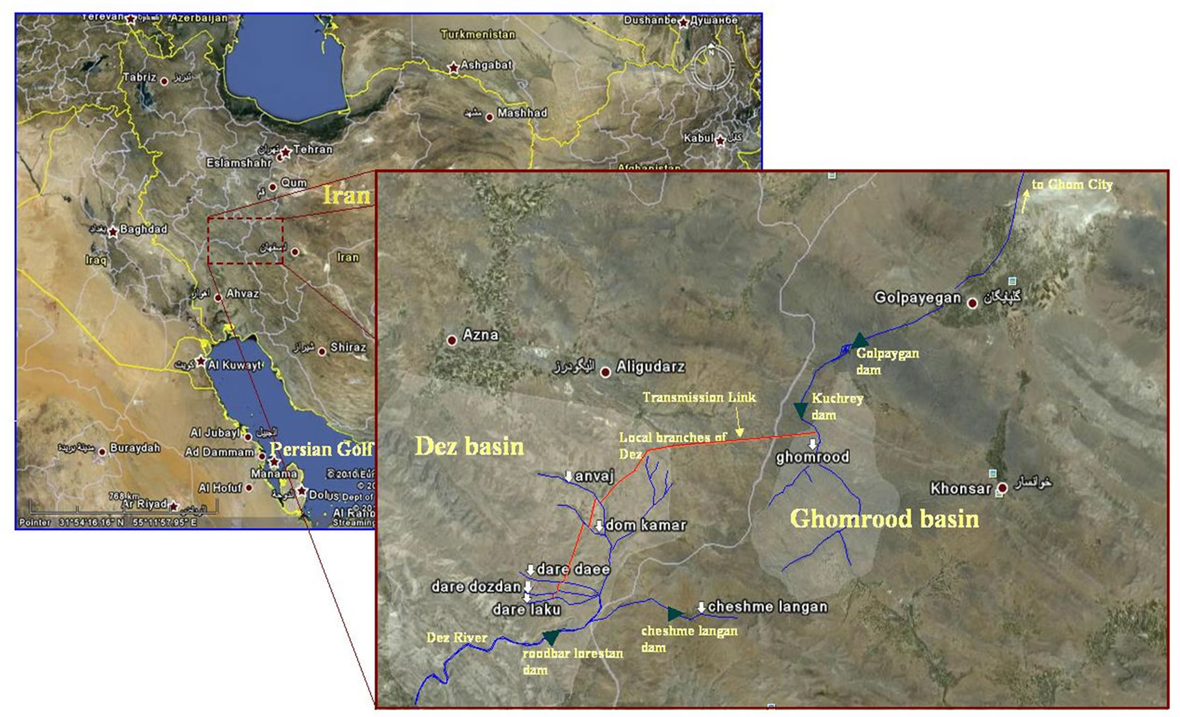
Figure 1. General geographic location, cells, and microcells which are generated in Dez and Qomrood basins by MAGICCSCENGEN.
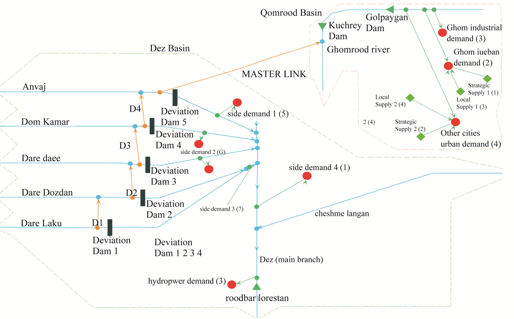
Figure 2. Schematic scheme and view of allocation model’s interface window of Dez to Qomrood water transmission project, more information are shown in Table 1.
house-gas Induced Climate Change) and its Nineteen GCMs have been used to calculate the change of precipitation in global scale. The resolution of MAGICCSCENGEN is a mesh of 2.5 × 2.5 degree cells. Figure 1 shows that how forty eight 2.5 × 2.5 degree cells covers Iran and environs, while Dez and Qomrood basins are located in no.19 and no.20 cells. Clearly, the GCMs cannot resolve the spatial structure of climate at the subbasin scale used in the hydrological model. To down scaling precipitation changes in local scale we used reverse-distance factors by utilizing results of neighboring cells given from GCMs in global scale. This method is applied by Andersson et al. to down scale precipitation results of GCMs on Okavango River basin [5]. To forecast monthly-scale precipitation, we have used GCMs results for monthly variation and compared these with historical monthly distribution to approach a basic monthly distribution function for each GCM-GHE scenario. Mitchell et al. have employed this method to forecast Europe and the globe climate factors [12]. In order to make more detailed grid network in the basin area, a minor mesh involving 0.5 × 0.5 degree microcells was generated and was utilized for downscaling.
Forecasted precipitation is used to develop runoff characteristics by utilizing a rainfall-runoff model. In this research historical data of rainfall and flow have been applied to develop monthly flow generator via a linier equilibrium. These generators are used to develop runoff for stochastic series of rainfall. Such simplified models, linier or non linier, are employed in several researches to forecast runoff in similar cases. Gardner employed exponential equilibrium to assess annual runoff in catchments with a wide range of climatic conditions [13]. This method also has been applied by a wide range of researchers like Graham, Chen, Benestad, and Carter [14- 17]. It’s very clear that many factors like land use, agriculture and irrigation patterns which have effects on basin’s hydrologic conductivity, are variable in long time. However, in this level of research scope, these uncertainties are inevitable and we neglect their impacts.
Table 3 illustrated final results for all GCM-Scenario combinations for 2050. In this research, the results of GCM-GHE scenarios have been classified in five groups Including Very Optimistic, Optimistic, Moderate, Pessimistic, and Very Pessimistic forecasting. Each group is weighted by the proportion of its GCM-GHE combinations to the whole probable space (see Table 2). All these GCMs have been used in IPCC Third Assessment Report (TAR). One GCM of each family is selected as a demonstrator of the group behavior. As it is shown in the Table 2, GCMs that we used in research are: GFDLCM-2.0, GISS-EH, UKHAD-GEM, GFDLCM-2.1 and FGOALS- 1G. Final results are Conformable with Third Assessment Report (TAR) generally. More than 68% of GHEGCM scenarios result a reduction between 6 to 28 percent in rainfall and consequently in the same order for runoff (see Table 3). TAR assesses reduction between 10 to 40 percent for 2090-2099 duration, relative to 1980
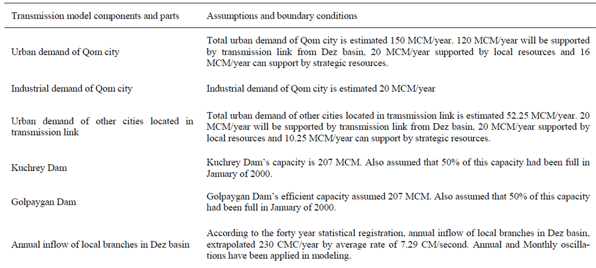
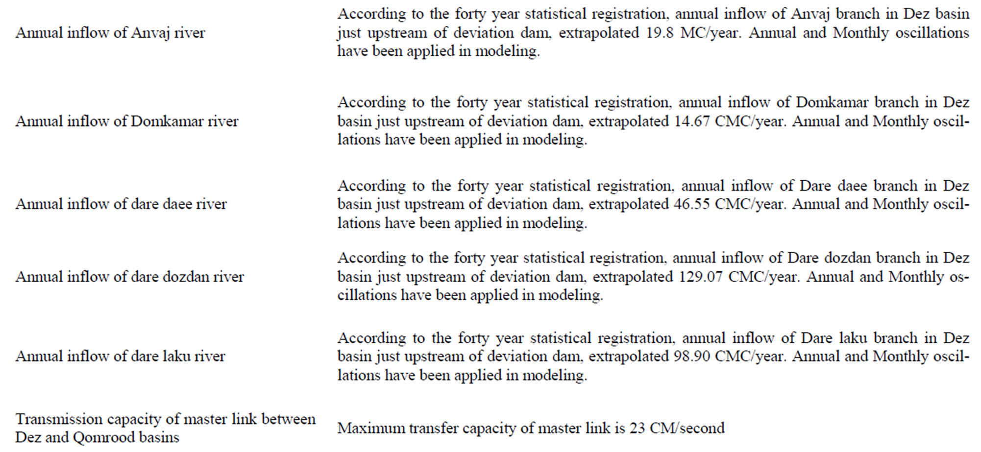
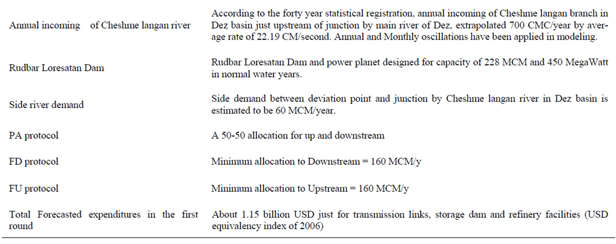
Table 1. Assumptions and boundary conditions applied in Dez to Ghomrood (Qomrood) water transmission model.
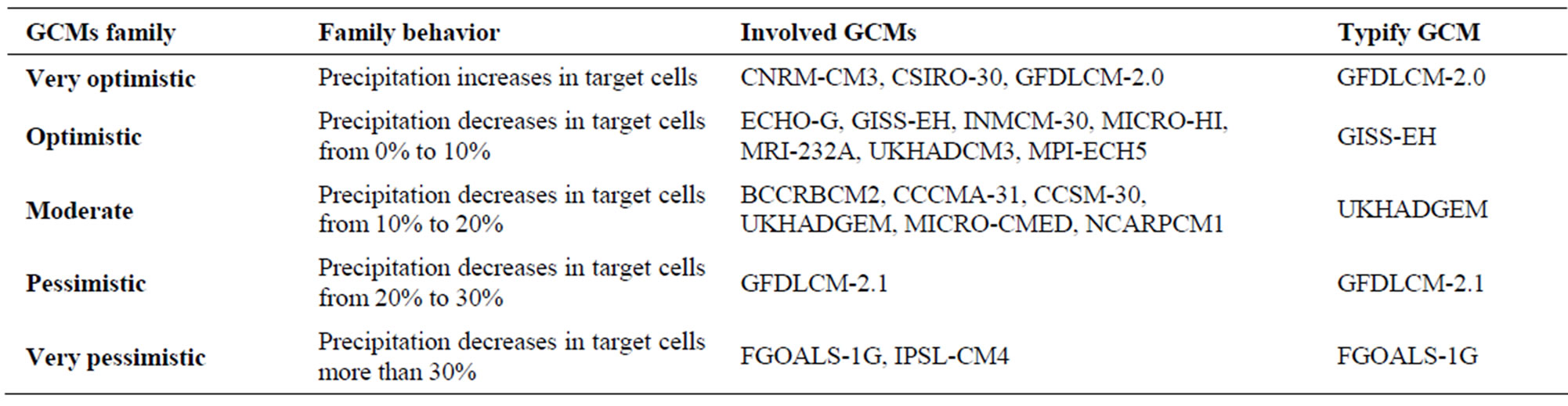
Table 2. GCMs families and their definitions in this research.
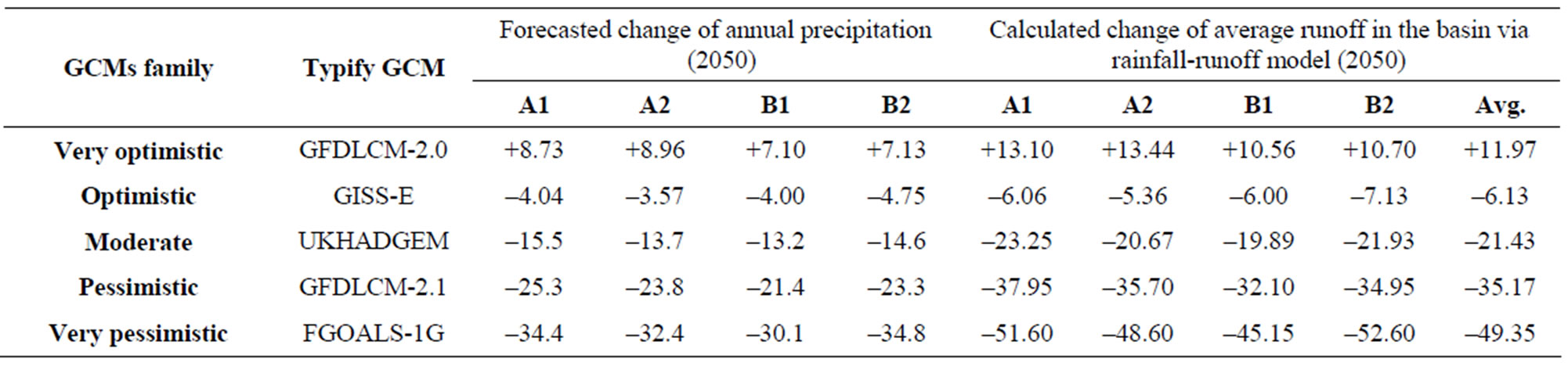
Table 3. Results of GCMs for precipitation and derived runoff in basin scale.
-1999. If this reduction happens in a linier pattern, decrease rate will be something between 5 to 20 percent for 2050 horizon. It can be a great confirmation for general results given by medium of GCMs. IPCC results are shown in Figure 3 [18,19].
3. Water Allocation Model and Water Transmission Protocols
In this paper, Water Evaluation and Planning (WEAP) have been used as a tool to model the basins. Mathematic equations were applied for modeling water transmission protocol as controllable valves in master transmission links. Table 1 illustrates initial figures and boundary conditions of the model. The model runs five GCMs outputs, four different climate scenarios and three transmission protocols. In this research, we analyzed three common sharing rules which have been described by Ansink & Ruijs [20]. General form of these Protocols and their policies are shown below:
Proportional Allocation (PA): upstream users receives αQt and downstream users receives (1 − α) Qt, with 0 < α < 1;
Fixed Upstream Allocation (FU): upstream users receives min {β, Qt} and downstream users receives Max {Qt −β, 0}, with 0 < β< E (Qt);
Fixed Downstream Allocation (FD): upstream users receives max {Qt − γ, 0} and downstream users receives Min {γ, Qt}, with 0 <γ < E (Qt).
In this definition, upstream is defined as the basin which can control transferred flow and downstream is the
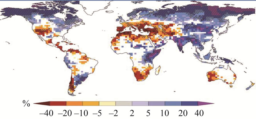
Figure 3. Large-scale relative changes in annual runoff for the period 2090-2099, relative to 1980-1999 [18]. White areas are where less than 66% of the ensemble of 12 models agreed on the sign of change, and hatched areas are where more than 90% of models agree on the sign of change.
basin which cannot control it. It is clear that water transmission projects and its policies are strongly related to socio-economic and politics indicators. This fact obviously can be seen in big and governmental projects, where politic force is the most important factor to stimulate the project [21]. Thus in such cases, like Dez to Qomrood water transmission project in Iran, due to government domination, all controls are under power of central government, however, in this research we assume principle basin (Dez) as upstream and destination basin (Qomrood) as downstream.
4. Results of Water Allocation Model
Despite the lack of fully reliable climate predictors in the project scale, an overwhelming majority of decision makers tend to have tangible results from climate predictions; one solution to this problem is to offer a series of weighted predictions developed by various aspect of climate prediction science. In order to gain clear results, final result should be interpreted by logical indexes which contain some sort of sustainability and analogical figures. Three tangible indexes are defined here to evaluate the efficiency of three water transmission protocols. The indexes are based on water and energy themes of CSD Indicators of Sustainable Development of UN with considering total population who gain benefits from the project [22]. These indicators are shown in Table 4.
Table 5 shows the final results of PA, FU, and FD transfer protocols for the three sustainability indexes and for A1-AIM scenario. In this table, we have considered the weight of each GCMs family based on climate prediction science to get more clear results. In these predictions we assume a series of Per-Capita indexes which will be used in next calculations. As it can be inferred from Table 3, a notable result of GHE-GCM models is that in this region the final results strongly depend on GCMs and the effect of climate scenarios is ignorable. Consequently the results are illustrated just for A1-AIM climate scenario and results gained from other climate scenarios are omitted in order to save the reader’s time. A swift glance on the final results shown on Table 5 indicates that there are significant differences between the performances of different protocols in each specific sector. All these three allocation protocols (Fix downstream, Fix upstream, and Proportional allocation) cause similar figures for hydroelectric section which may happen owing to the location of the power planet supplied by the other branches from the eastern part of Dez basin. For agriculture sector, there is a considerable difference between the result of FU and other protocols, but the most significant variance is observed for the urban demand. More than 2,424,000 of people will be supplied by standard per capita fresh water if FD protocol is selected. The figure shows 2,123,000 for PA protocol and 2,013,000 people for FU. Furthermore, total supplied people by the system exceed more than 2,875,000 for FD protocol, considerably more than 2,576,000 and 2,480,000 for PA and FU respectively. As a common rule, Fix allocation to the main basin (in this case FU) has the minimum disrupting effects on a hydrologic system in comparison with the other protocols. In addition, FU protocol contains less social conflicts than other protocols because it ensures a minimum flow for the main basin in which stakeholders can’t adapt themselves easily with instance changes caused by the project. The figures illustrated in Table 5 are provided by probability diagrams which are directly produced by water allocation model. As a sample, Probability diagram for the volume of transferred water is shown in Figure 4.
By considering a budget about 1.15 billion US$ for the project, Table 6 illustrates people who will be covered by different aspects of welfare indexes for each 1000 US$ investment in the project. These figures don’t contain second round of expenditure like social issues and real cost of environmental damages of construction and operation. But as a swift glance they provide figures for a constructed project which is exist willy-nilly.
5. Conclusion
If we just focus on total supported population, FD proto-

Table 4. Comprehensive indexes which have been used in this research, based on “UN: Indicators of sustainable development” definitions [22]. Per-capita indexes are shown in the last column are taken from different resources.
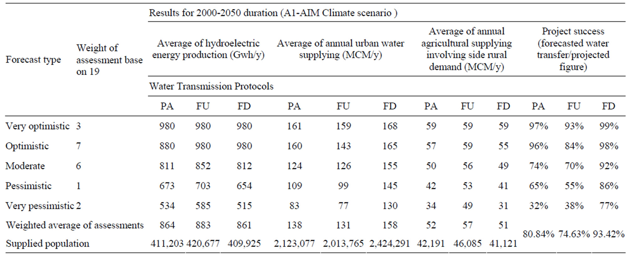
Table 5. Results of sustainable indicators for FD protocol in face climate change in dez to Qomrood water transmission project, 2000-2050 duration, A1-AIM climate scenario.
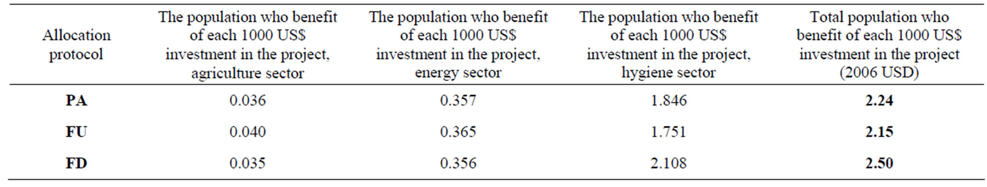
Table 6. The population who make a profit of different aspects of welfare for each 1000 USD investment in the water transfer project.
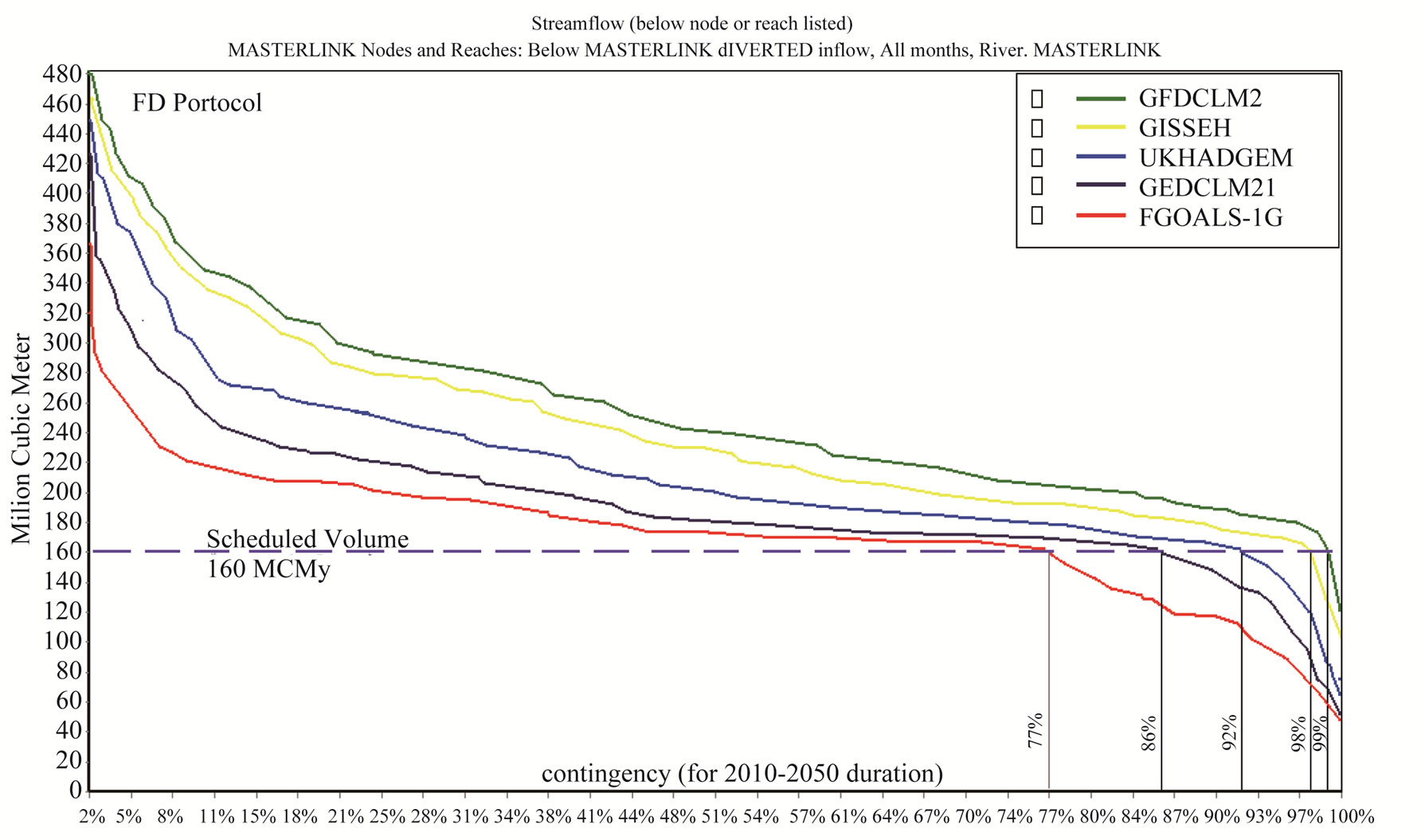
Figure 4. Water transfer probability diagram for Fix Downstream (FD) allocation protocol (time period 2010-2050). As it is shown in the graph, the project has been designed to transfer a volume of 160 MCM/y. This is the base for related results of Table 5. Similar diagrams were developed for other sectors.
col will supply a larger group of people. However, PA and FU protocols will put a slighter pressure on the stakeholders who live in the main basin. As a conclusion, there is a tradeoff between the benefit and difficulties of each protocol, but if the economic costs of the project are considered, FD protocol will illustrate its efficiency besides more supplied people. FD protocol will achieve more than 93% of the project’s aim in duration from 2010 to 2050 whereas Table 5 shows 80.84% and 74.63% for PA and FU. Current results are rational because FD protocol focuses on maximum possible water transmission in this case; while FU protocol looks for minimum water transmission and PA has a moderate behavior. This research contains the result of the first layer of climate change impacts and a governmental project with considering its special limits. It’s recommended to Future researches to focus on the second layer of socio-economic affairs and consider real cost of project as an effective item. In addition, some social issues like immigration to constructed areas and effects of new reservoirs, rate of job cutting, governmental subsides on agriculture and hydropower and other factors should be considered. These factors are important to develop an unbiased model which can help water resources managers to have a clear image of the future, and have a multi-criteria knowledge about the real cost and benefits of each protocol.
REFERENCES
- G. J. van Oldenborgh, F. J. Doblas-Reyes, B. Wouters and W. Hazeleger, “Skill in the Trend and Internal Variability in a Multi-Model Decadal Prediction Ensemble,” Climate Dynamics, Vol. 3, No. 7, 2012, pp. 1263-1280. doi:10.1007/s00382-012-1313-4
- Y. Chikamoto, M. Kimoto, M. Ishii, T. Mochizuki, T. Sakamoto, H. Tatebe, Y. Komuro, M. Watanabe, T. Nozawa, H. Shiogama, M. Mori, S. Yasunaka and Y. Imada, “An Overview of Decadal Climate Predictability in a Multi-Model Ensemble by Climate Model MIROC,” Climate Dynamic, 2012.
- H. Kunstmann, G. Jung, S. Wagner and H. Clotte, “Integration of Atmospheric Sciences and Hydrology for the Development of Decision Support Systems Sustainable Water Management,” Physics and Chemistry of the Earth, Vol. 33, No. 1-2, 2008, pp. 165-174. doi:10.1016/j.pce.2007.04.010
- A. Serrat-Capdevila, J. B. Valdésa, J. G. Péreze, K. Baird, J. Mafa and T. Maddock, “Modeling Climate Change Impacts and Uncertainty on the Hydrology of a Riparian System: The San Pedro Basin (Arizona/Sonora),” Journal of Hydrology, Vol. 347, No. 1-2, 2007, pp. 48-66. doi:10.1016/j.jhydrol.2007.08.028
- L. Andersson, J. Wilk, M. C. Todd, D. A. Hughes, A. Earle, D. Kniveton, R. Layberry and H. G. Savenije, “Impact of Climate Change and Development Scenarios on Flow Patterns in the Okavango River,” Journal of Hydrology, Vol. 331, No. 1-2, 2006, pp. 43-57. doi:10.1016/j.jhydrol.2006.04.039
- A. Wolf, “Conflict and Cooperation along International Waterways,” Water Policy, Vol. 1, No. 2, 1998, pp. 251- 265. doi:10.1016/S1366-7017(98)00019-1
- M. Giordano and A. Wolf, “Sharing Waters: Post-Rio International Water Management,” Natural Resources Forum, Vol. 27, No. 2, 2003, pp. 163-171. doi:10.1111/1477-8947.00051
- R. Ghanadan and J. B. Koombey, “Using Energy Scenarios to Explore Alternative Energy Pathways in California,” Energy Policy, Vol. 33, No. 9, 2005, pp. 1117-1142. doi:10.1016/j.enpol.2003.11.011
- A. Oniszk-Poplawska and M. Rogulska, “RenewableEnergy Developments in Poland to 2020,” Applied Energy, Vol. 1-3, No. 76, 2003, pp. 101-110. doi:10.1016/S0306-2619(03)00051-5
- M. Eames, “The Development and Use of the UK Environmental Future Scenarios: Perspectives from Cultural Theory,” Greener Management International, Vol. 37, 2002, pp. 53-70.
- K. Ito and Y. Uchiyama, “Study on GHG Control Scenarios by Life Cycle Analysis—World Energy Outlook until 2100,” Energy Conversion and Management, Vol. 38, 1997, pp. 607-614. doi:10.1016/S0196-8904(97)00004-6
- T. D. Mitchell, T. R. Carter, P. D. Jones, M. Hulme and M. New, “A Comprehensive Set of High-Resolution Grids of Monthly Climate for Europe and the Globe: The Observed Record (1901-2000) and 16 Scenarios (2001- 2100),” Tyndall Centre Working Paper No. 55, 2004.
- L. R. Gardner, “Assessing the Effect of Climate Change on Mean Annual Runoff,” Journal of Hydrology, Vol. 379, No. 3-4, 2009, pp. 351-359. doi:10.1016/j.jhydrol.2009.10.021
- L. Graham, J. Andréasson and B. Carlsson, “Assessing Climate Change Impacts on Hydrology from an Ensemble of Regional Climate Models, Model Scales and Linking Methods: A Case Study on the Lule River Basin,” Climate Change, Vol. 81, 2007, pp. 293-307. doi:10.1007/s10584-006-9215-2
- D. L. Chen, et al., “Using Statistical Downscaling to Quantify the GCM-Related Uncertainty in Regional Climate Change Scenarios: A Case Study of Swedish Precipitation,” Advances in Atmospheric Sciences, Vol. 23, 2006, pp. 54-60. doi:10.1007/s00376-006-0006-5
- R. E. Benestad, “Tentative Probabilistic Temperature Scenarios for Northern Europe,” Tellus Series A: Dynamic Meteorology and Oceanography, Vol. 56, 2004, pp. 89-101.
- T. R. Carter, et al., “Developing and Applying Scenarios in Climate Change: Impacts, Adaptation, and Vulnerability IPCC,” Cambridge University Press, Cambridge, 2001, pp. 145-190.
- P. C. D. Milly, K. A. Dunne and A. V. Vecchia, “Global Pattern of Trends in Streamflow and Water Availability in a Changing Climate,” Nature, Vol. 438, No. 7066, 2005, pp. 347-350. doi:10.1038/nature04312
- B. C. Bates, Z. W. Kundzewicz, S. Wu and J. P. Palutikof, “Climate Change and Water. Technical Paper of the Intergovernmental Panel on Climate Change, IPCC Secretariat,” Geneva, 2008.
- E. Ansink and A. Ruijs, “Climate Change and the Stability of Water Allocation Agreements,” Environmental and Resource Economics, Vol. 41, 2008, pp. 133-287. doi:10.1007/s10640-008-9190-3
- B. Gumbo and P. van der Zaag, “Water Losses and the Political Constraints to Demand Management: The Case of the City of Mutare, Zimbabwe,” Physics and Chemistry of the Earth, Vol. 27, No. 11-22, 2002, pp. 805-813. doi:10.1016/S1474-7065(02)00069-4
- United Nations, “Indicators of Sustainable Development: Guidelines and Methodologies,” 3rd Edition, United Nations, New York, 2007.