Journal of Water Resource and Protection
Vol. 2 No. 10 (2010) , Article ID: 2965 , 8 pages DOI:10.4236/jwarp.2010.210105
Development of Flood Forecasting System Using Statistical and ANN Techniques in the Downstream Catchment of Mahanadi Basin, India
1Department of Hydrology, Indian Institute of Technology, Roorkee, India
2National Institute of Hydrology, Roorkee, India
3Department of Water Resources, Government of Orissa, Bhubaneswar, India
E-mail: aklnih@gmail.com, lohani@nih.ernet.in
Received May 6, 2010; revised July 27, 2010; accepted August 12, 2010
Keywords: Flood Forecasting, Mahanadi Basin, Hirakud Dam, Statistical Method, ANN Architecture, Clustering
ABSTRACT
The floods in river Mahanadi delta are due to either dam release of Hirakud or due to contribution of intercepted catchment between Hirakud dam and delta. It is seen from post-Hirakud periods (1958) that out of 19 floods 14 are due to intercepted catchment contribution. The existing flood forecasting systems are mostly for upstream catchment, forecasting the inflow to reservoir, whereas the downstream catchment is devoid of a sound flood forecasting system. Therefore, in this study an attempt has been made to develop a workable forecasting system for downstream catchment. Instead of taking the flow time series concurrent flood peaks of 12 years of base and forecasting stations with its corresponding travel time are considered for analysis. Both statistical method and ANN based approach are considered for finding the peak to reach at delta head with its corresponding travel time. The travel time has been finalized adopting clustering techniques, there by differentiating high, medium and low peaks. The method is simple and it does not take into consideration the rainfall and other factors in the intercepted catchment. A comparison between both methods are tested and it is found that the ANN methods are better beyond the calibration range over statistical method and the efficiency of either methods reduces as the prediction reach is extended. However, it is able to give the peak discharge at delta head before 24 hour to 37 hour for high to low peaks.
1. Introduction
Flood is a regular phenomenon in the delta of Mahanadi basin. The discharge of the intercepted catchment of below Hirakud dam has contributed largely to the flood at delta. The delta is highly fertile and thickly populated with population density 400-450 persons per sq.km. The drainage capacity of deltaic rivers is 25500 m3/s only. Any discharge above this can create a flood like situation.
Establishment of a workable flood forecasting method for the downstream catchment of Mahanadi basin is always under scanner. A lot of hydro-meteorological information is needed for establishment of a model. The dam at upstream is operated by a rule curve. The intercepted catchment is very big around 40000 sq.km. In order to establish a Rainfall-Runoff model, rainfall data of all station is highly essential. For further strengthening of model evaporation, soil moisture, temperature, dam release etc. are needed. Sometimes all information is not available on real time basis making it difficult for establishment of a physical based model. In that case statistical methods are more useful.
The statistical methods are generally graphical or in the form of mathematical relationship, developed with the help of historical data, using statistical analysis. These include simple gauge to gauge relationships, gauge to gauge relationship with additional parameters and rainfall-peak stage relationship. These relationships can be easily developed and are most commonly used in India as well as other countries of the world [1]. Spokkerreff [2] has mentioned about application of statistical model till 1995 on river Rhine.
Consequently, there is need for models capable of efficiently forecasting water levels and discharge rates. In this regard application of ANN is more effective. Earlier the works of Bruen and Yang [3], Campolo et al. [4,5], Coulibaly et al. [6], Dawson and Wilby [7], Imrie et al. [8], Lekkas et al. [9], Lohani [10], Minns and Hall [11], Muhamad and Hassan [12], Mukerji et al. [13], Solomantine and Xue [14], Solomantine and Price [15], Zealand et al. [16] emphasized the application of artificial neural networks over other methods. In flood forecasting both the peak and travel time has equal significance. The travel time is also of great importance in prediction of the stage. It varies with stages and channel condition. Travel time generally reduces when water approaches the top of the bank. As the river overflows flooding over the flood plain the travel time may begin to increase again due to the relatively rough surfaces lying in the overbank stages. In order to give justification for different types of peaks with respect to travel time clustering method is adopted in this study. Earlier, Zhang and Hall [17] have applied clustering methods in regional flood frequency analysis and Xiongrui et al. [18] in establishing rainfallrunoff relationships. In view of the above an attempt has been made in this study to apply both statistical method and ANN based approach for forecasting the peak discharge and travel time in the downstream reach of the Mahanadi River.
2. Study Area
The Mahanadi basin lies between 800-30` to 860-50` of East Longitude and 190-20` to 230-35` of North Latitude. The river Mahanadi is an interstate river. The catchment area of the basin is 141569 sq. km. The major part of this catchment lies in Chhatisgarh (75136 sq. km.) (Figure 1). As this part is the upstream part, 143 channels in this zone generally feeds the Hirakud reservoir having a catchment of 83400 sq.km. The downstream catchment has three main tributaries like Jeera, Ong and Tel with catchments 2383, 5128 and 25045 sq.km. respectively. So the contributions from the Tel catchment always remain predominant. Even the flood of 2008 is mainly due to the contribution of this tributary. It has produced a peak discharge of 33762 cumecs during 2008. So establishment of a flood forecasting model below the joining of these tributaries reduces the ambiguity. The river Tel joins at Patharla to the main river Mahanadi and our base station Khairmal is at downstream of Patharla station. The other tributaries Ong and Jeera join also at the upstream of base station (Khairmal). The whole river from Khairmal is taken as one unit ignoring the contribution of further small tributaries. A schematic presentation shows the distance and travel time from Hirakud to Mundali presently being used for the official purposes of Department of Water Resources, Government of Orissa [19].
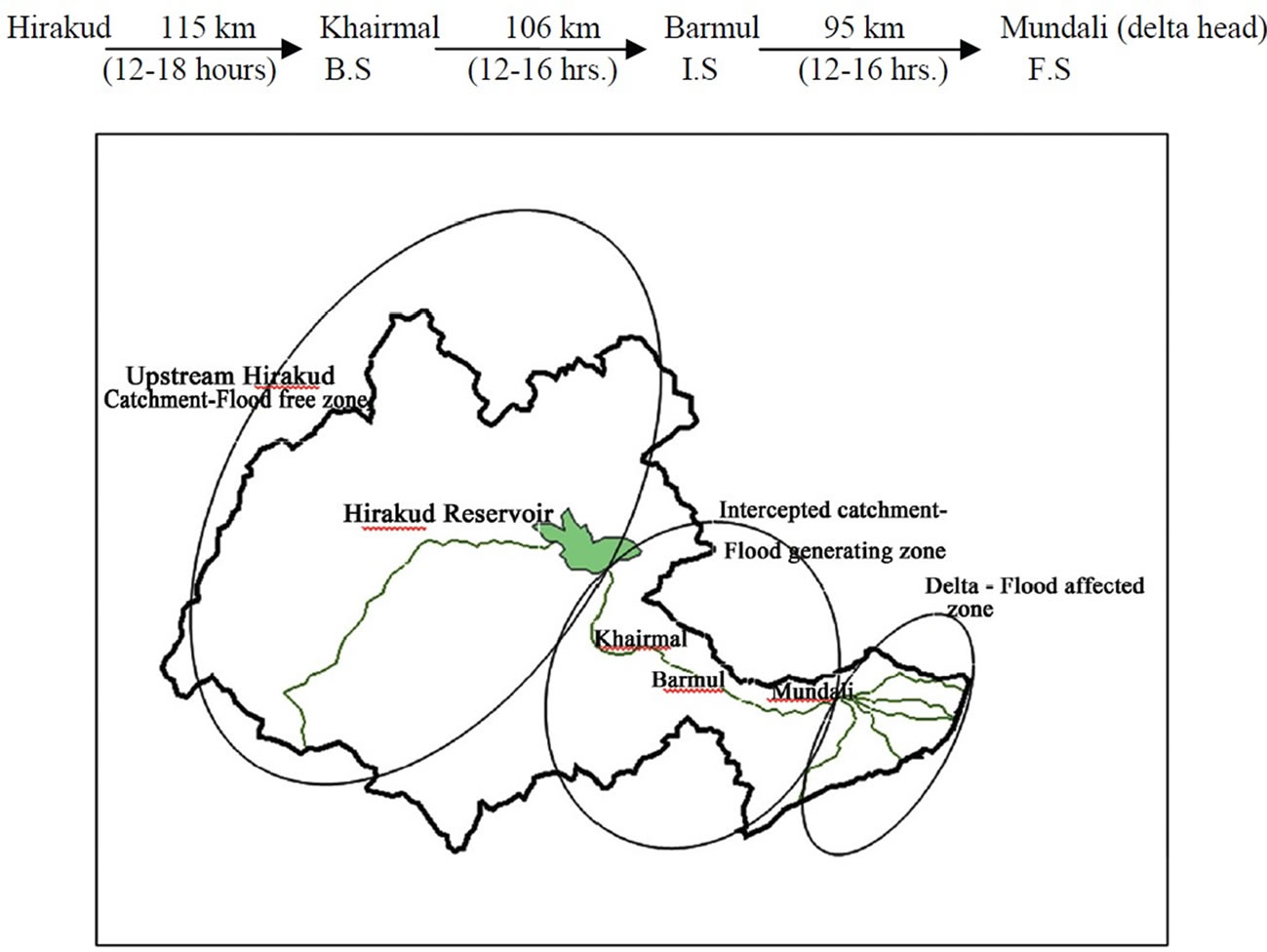
Figure 1. Showing catchment details with different zones of Mahanadi basin.
In our study the station at Khairmal is taken as the base station (B.S) which is 115 km away and with an average lead time of 12-16 hour for Hirakud release to reach here. Barmul is the intermediate station (I.S) and Mundali is the forecasting station (F.S) just upstream of Cuttack city.
3. Data Availability
Adequate data is needed for the formulation of the forecasting services. The development of the river forecasting procedure requires historical hydrological data and for the preparation of operational forecasts sufficient current information is required. Discharge data of (3 hourly) is available at base, intermediate and forecasting station for a period of 1996-2007. Discharge of 2830 cumecs and above at forecasting stations are considered as peaks and its corresponding peaks at intermediate and base station are collected with their related travel times after drawing the corresponding time series. Out of this 80 peaks are considered for our analysis, taking 60 peaks for calibration and 20 peaks for testing of models. Generally, it can be said that it is necessary to have a minimum of 10 years of basic hydraulic data, available to develop adequate river forecasting procedures, the primary requirement being that the period of record should contain a representative range of peak flows [20].
4. Methodology
The selection of an appropriate flood forecasting model depends on the availability of the data, output desired etc. On the basis of the analytical approach for the development of flood forecasting method can be classified as:
1) Methods based on statistical approach.
2) Methods based on mechanism of formation and propagation of floods.
4.1. Statistical Approach
Finding correlation between stage and discharges between upstream and downstream gauging stations is one of the simplest methods. This gives better result when there is less influence of tributaries joining the main stream in between or the intercepted catchment is not influenced by heavy rainfall.
4.2. ANN Approach
There are many ANN architectures and algorithms developed. Out of them most common are Multi layer feed forward, Hoppfield networks, Radial basis function network, Recurrent network, Self organization feature maps, Counter propagation networks. Selection of a particular network is application oriented. However, the multi layer feed forward networks are most commonly used for hydrological applications [7].
Generally four distinct steps applied to any ANN – based solution including flood forecasting problems. First of all data transformation is the initial step. The input always varies in a larger range. So in order to lessen the range the data is put in logarithmic scale. Then normalization and scaling is done. Data sets with many variations make training difficult. In order to prevent it the data are usually scaled using statistical, min-max, sigmoidal or principal component transformations [21]. Also the absolute input values are scaled to avoid asymptotic issues [22].
The second step is the fixing the network architecture in which for a particular problem the number of hidden layers, neurons in each layer and the connectivity between neurons are set. Many experimental results say that one hidden layer may be enough for most forecasting problems [6,17]. The studies of Cybenko [23], Hornik et al. [24] revealed that a single hidden layer is sufficient for ANNs to approximate any non-linear transfer function. The number of neurons in each layer depends upon the problem being studied. Less number of neurons in hidden layer will make the network with less degree of freedom for learning and more number of neurons will lead towards more time and over fitting [25]. Validation set error is often used to determine the optimal number of hidden neurons for a given study.
In the third step is the finalization of a learning algorithm for training the network. The parameters are finalized for the training data set to be applicable for any kind of testing data. ANN architecture is considered to be trained when the difference between ANN output and observed output is very small.
Finally the validation step is applied to get the performance of the network. The optimal number of hidden neurons and training iterations can also be determined through validation. The selection of acceptable model is finalized on the basis of RMSE, R2 and efficiency.
4.3. Clustering Approach
As the data set varies in a wide range, it requires some distinction and in particular when different peaks are available for the same travel time. In order to make proper justice for different peaks with respective travel time, it requires clustering. Both K-mean and Fuzzy C-mean clustering methods are attempted.
4.3.1. K-Mean
This method was developed by MacQueen [26]. It is best described as a partitioning method. It partitions the data into K mutually exclusive clusters and returns a vector of indices indicating to which of the K-clusters it has assigned each observation. The algorithm to clusters N objects based on attributes into K partitions where K < N. The optimization function
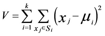 (1)
(1)
It tries to achieve minimum intra cluster variance or the squared error function. Where there are K clusters Si = 1,2……K, and Vi is the centroid or mean point of all the points Xj Є Si. [27].
4.3.2. Fuzzy C-Mean (FC)
In this method the affinity of a site to undergo either two or more clusters are visualized. Earlier developed by Dunn [28] and improved by Bezdeck [29] is basically used for pattern recognition. Here the data are bound to each cluster by means of a membership function which represents the Fuzzy behavior of this algorithm. It shows how to group data points that populate some multidimensional space into a specific number of different clusters. The objective function
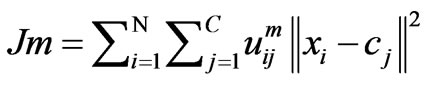 ,
, (2)
(2)
 = any real number,
 = degree of membership of
  in cluster
 ,
,  = ith of d-dimensional measured data,
 = d-dimension center of cluster.
Similarly, different ANN architectures are attempted over the discharge and corresponding travel times. The calibration and validation data sets remain same for both the methodology. The same methodology is also adopted for finding the travel time. But in order to further distinguish K-mean and Fuzzy C mean clustering methods are adopted to find a better answer for travel time of different peaks.
5. Results and Discussion
First of all statistical approach is applied into calibration dataset (60 nos.). The relationships between the discharges between Khairmal-Barmul, Barmul-Mundali, Khairmal-Mundali and Khairmal-Barmul-Mundali are developed. These relationships are put on the testing data sets (20 nos.) and the results are recorded in Table 1.
Where, QM = discharge at Mundali (Forecasting Station), QB = discharge at Barmul (Intermediate Station) and QK = discharge at Khairmal (Base Station).
The same dataset is again put into ANN architecture using MATLAB codes. The trial has been taken with a 3-layer feed forward network. Different combinations of feed forward network with changing transfer function, number of neurons and epochs varying at an increment of 50 are trailed. The combinations which are mostly as per performance criteria fixed are noted. The Cascade feed forward network has been most successful for Khairmal-Barmul and Khairmal-Barmul-Mundali and other two cases are with Feed forward network. Numbers of neurons in input and output layers are mentioned in column (2) of Table 2. In all cases ‘tansig’ neurons are used in first layer, ’purelin’ in second layer and ‘trainbr’ remains the training function. Both ‘tansig’ and ‘purelin’
are better compatible with feed forward networks. Again the two layer sigmoid/linear network can represent any

Table 1. Relationship between discharges using simple statistical method (peak to peak).
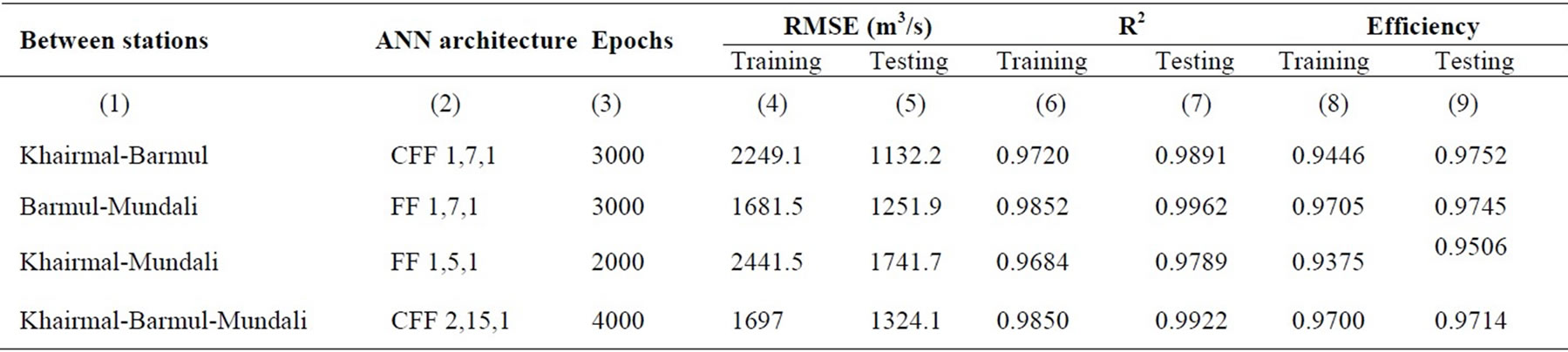
Table 2. Relationship between discharges using ANN architecture.
functional relationship between inputs and outputs if the sigmoid layer has enough neurons [30]. The ‘trainbr’ function updates the weight and bias values as per Levenberg-Marquardt optimization. It minimizes the combination of squared errors and weights and then determines the correct combination so as to produce a network that generalizes well as per Bayesian regularization process. It reduces the difficulty of determining the optimum network architecture also over fitting of training dataset is prevented, whereas in other networks generalization and early stopping is required for reducing over fitting. The performance functions are set as RMSE, R2 and efficiency. The details of the network applied for different combinations are shown in Table 2.
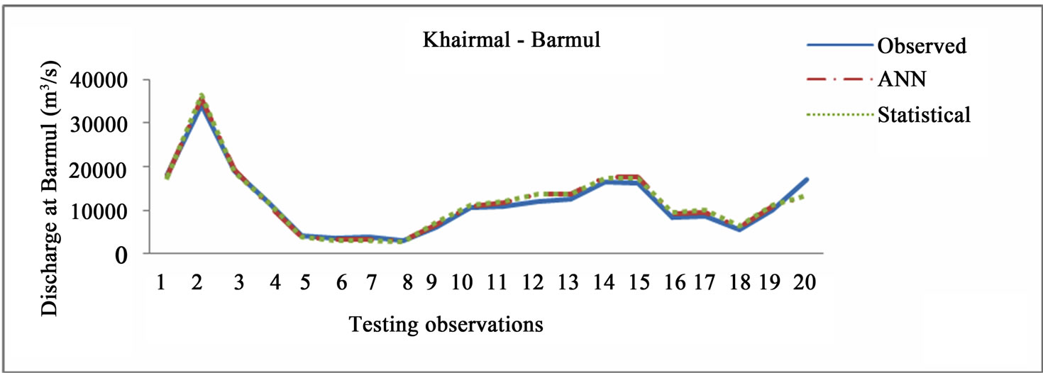
The plots of the statistical method and ANN network over the testing value of 20 numbers of observation as obtained from MATLAB is also produced in Figures 2(a) to (d) respectively.
For travel time the corresponding discharge and travel times between the stations are trailed with the same calibration and testing data range applying both Statistical (Table 3) and ANN architectures (Table 4). The ANN is also applied in the same way with many numbers of trials.
It has been revealed that none of the case has a good efficiency, RMSE and R2. All the relations are ended with a poor correlation. The lack of correlation does not imply lack of association. Because ‘r’ measures only linear association, a strict curvilinear relationship would not necessarily be reflected in a high ‘r’ value. Conversely, correlation between two variables does not guarantee that they are causatively connected [31].
However, to have a better answer for efficiency and RMSE values clustering methods are adopted for the discharge value at base station and its corresponding travel time for the calibration dataset. At least 4 clusters are attempted applying K-mean and Fuzzy c-mean method using the same MATLAB code. The datasets are divided into 4 clusters and their varying ranges are recorded. For each range the average travel time has been calculated. In both methods low peak (2660-8256 m3/s) has large travel time (37.77 hours) to reach at delta head where as high peaks has taken nearly 25 hours to reach at delta head. As each peak is categorized the respective travel time for different discharge values are fixed. However when the result is put over the test dataset K-mean clustering has given 80% efficiency with RMSE value of 2.5 hour (Table 5). One value of testing dataset has been removed because it seems that it has some recording errors. So travel time test series has been carried out with 19 numbers of data.
A plot (Figure 3) has been drawn with observed test-
 (a)
(a)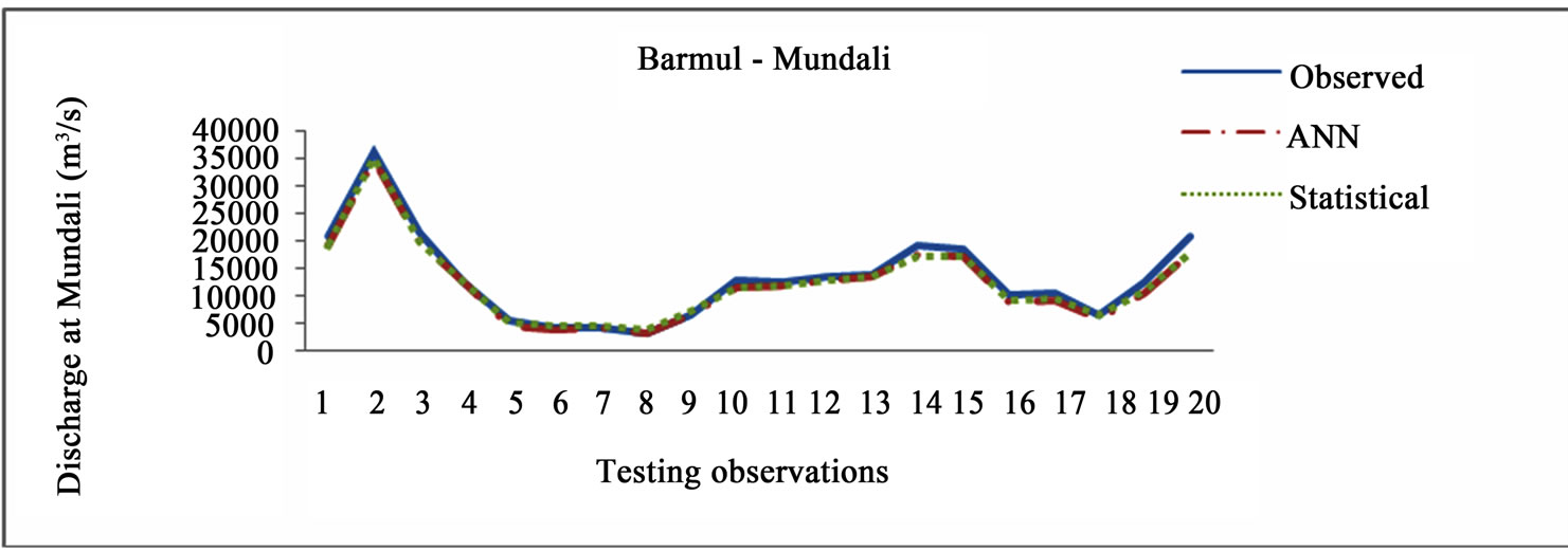 (b)
(b) (c)
(c) (d)
(d)
Figure 2. (a) Comparison between observed and computed discharge (Khairmal-Barmul); (b) Comparison between observed and computed discharge (Barmul-Mundali); (c) Comparison between observed and computed discharge (Khairmal-Mundali); (d) Comparison between observed and computed discharge (Khairmal-Barmul-Mundali).
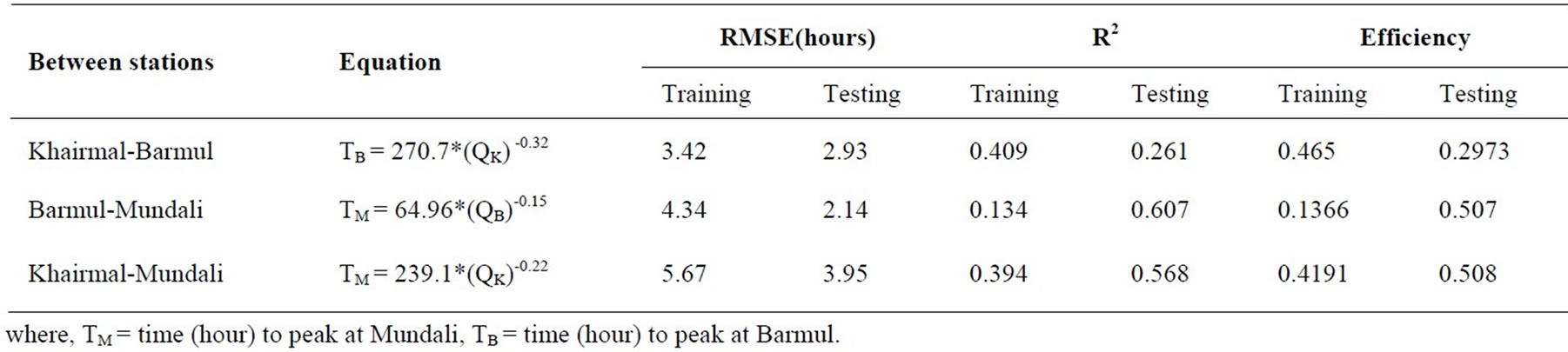
Table 3. Relationship between discharges and travel time using simple statistical method.
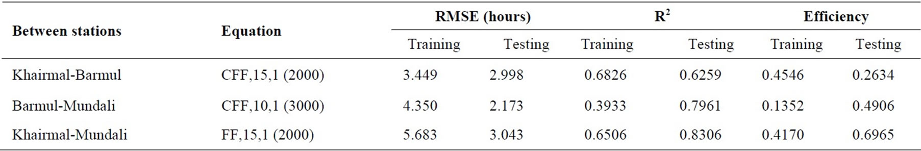
Table 4. Relationship between discharges and travel time using ANN.
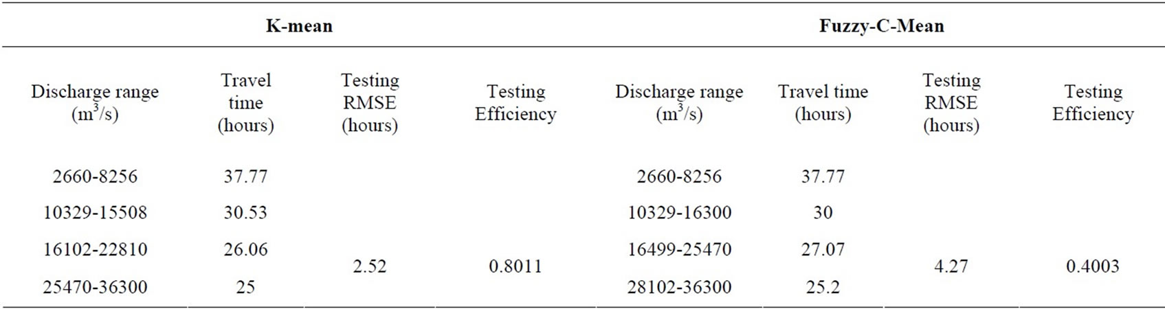
Table 5. Peak values with corresponding travel time obtained by using different clusteringmethods
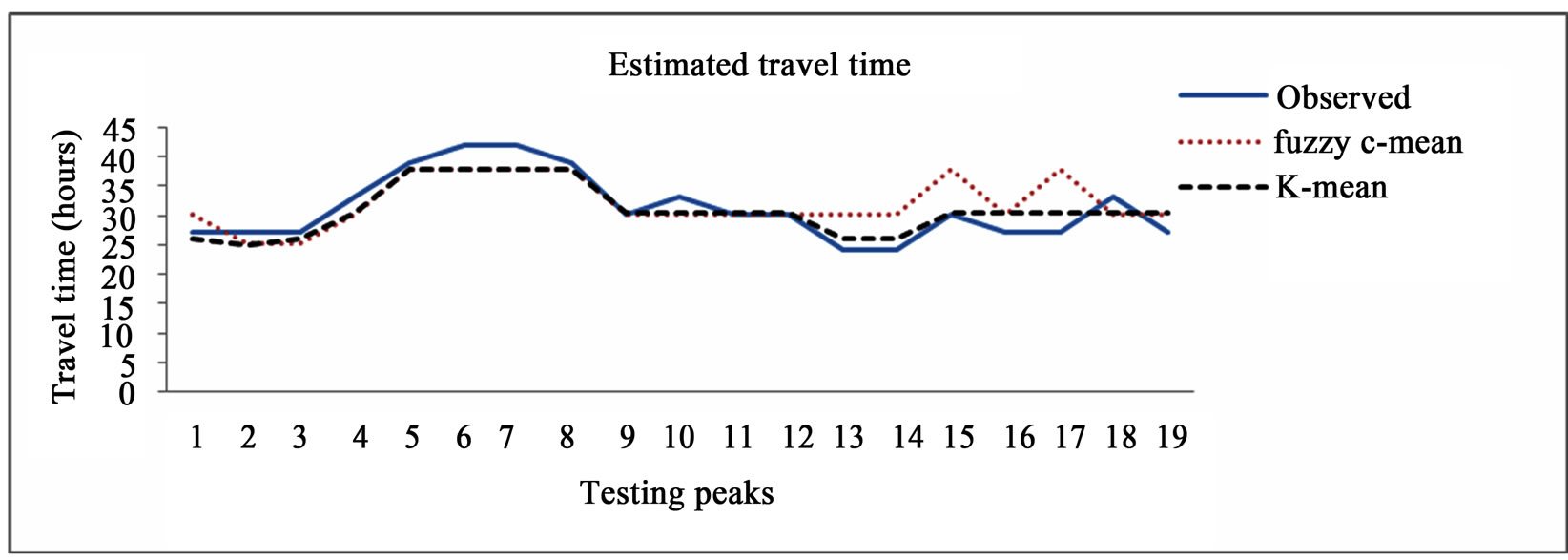
Figure 3. Plot between testing travel time and estimated by different clustering methods.
ing values and validation result of different clustering values. The plot shows the result of K-mean clustering is almost close with that of observed, whereas result of Fuzzy C mean for some low peak values. For high peaks both K-mean and Fuzzy have same results. As K-mean has able to model both high and low peaks with an efficiency of 80.1%,which is higher than Fuzzy C-mean methods, the discharge range values and its corresponding travel time fixed by this method may be taken as the forecast travel time between base station and forecasted station. The travel time has not calculated for other intermediate stations as our concentration is with the peak at base station and travel time of at least 24 hour.
6. Conclusions
Both statistical and ANN methods are applied for downstream Hirakud catchment between stations Khairmal, Barmul and Mundali. The forecasting obtained by both the methods is encouraging. Although the ANN method has a better performance, the existence of statistical method cannot be denied as far as discharge measurement is considered. However, the adoption of clustering method in order to find travel time with respect to different peaks is another finding. The best result for travel time is for Khairmal-Mundali reach (efficiency = 80.11% and RMSE = 2.55 hour). As the data recording is of 3 hour interval this kind of result is still encouraging. The travel time between base and forecasting stations varies between 24-37 hour. By applying clustering method justice has been made for different magnitude of peaks. The results are handy to operate. The moment one gets the discharge at Khairmal (Base Station), he can immediately calculate the discharge to be obtained at Mundali (Forecasting Station) with its corresponding travel time. The result at Mundali (Forecasting Station) with respect to Khairmal (Base Station) basing on the ANN network is best for taking the flood forecasting effectively because in taking Khairmal-Barmul and Barmul-Mundali efficiency is above 97% and RMSE value is 500 m3/s less than Khairmal-Mundali but lead time of only 12 hours remains after Barmul. So considering the factor of higher lead time for more relief measures we are making a tradeoff with efficiency. Thus calculating peak discharge and travel time at Mundali on the basis of Khairmal discharge and time of occurrence will be a best workable method for practicing hydrologists and field engineers. Still the results are running with the limitation of data insufficiency, large recording intervals, non-consideration of influence of other climatic variation.
REFERENCES
- Central Water Commission of India, “Manual on Flood Forecasting,” 1980.
- E. Spokkereff, “Flood Forecasting for the River Rhine in the Netherlands,” Proceeding of the Symposium the Extreme of Extremes: Extraordinary Floods, Reykjavic, Ireland, July 2000, pp. 347-352.
- M. Bruen and J. Yang, “Functional Networks in RealTime Flood Forecasting - A Novel Application,” Journal of Advances in Water Resources, Vol. 28, No. 9, 2005, pp. 899-909.
- M. Campolo, P. Andreeussi and A. Soldati, “River Flood Forecasting with a Neural Network Model,” Water Resources Research, Vol. 35, No. 4, 1999, pp. 1191-1197.
- M. Campolo, A. Soldati and P. Andreeussi, “Artificial Neural Network Approach to Flood Forecasting in the River Arno,” Hydrological Sciences Journal, Vol. 48, No. 4, 2003, pp. 381-398.
- P. Coulibaly, F. Anctil and B. Bobee, “Daily Reservoir Forecasting Using Artificial Neural Network with Stopped Training Approach,” Journal of Hydrology, Vol. 230, No. 3-4, 2000, pp. 244-257.
- C. W. Dawson and R. L. Wilby, “Hydrological Modeling Using ANN,” Progress in Physical Geography, Vol. 25, No. 1, 2001, pp. 80-108.
- C. E. Imrie, S. Durucan and A. Korre, “River Flow Prediction Using Artificial Neural Network: Generalization beyond the Calibration Range,” Journal of Hydrology, Vol. 233, No. 1-4, 2000, pp. 138-153.
- D. F. Lekkas, C. Onof, M. J. Lee and E. A. Baltas, “Application of Neural Networks for Flood Forecasting,” Global Nest: The International Journal, Vol. 6, No. 3, 2004, pp. 205-211.
- A. K. Lohani, “ANN and Fuzzy Logic in Hydrological Modeling and Flow Forecasting,” Ph.D Dissertation, Indian Institute of Technology, Roorkee, 2007.
- A. W. Minns and M. J. Hall, “Artificial Neural Networks as Rainfall-Runoff Models,” Hydrological Sciences Journal, Vol. 41, No. 3, 1996, pp. 399-417
- J. R. Muhamad and J. N. Hassan, “Khabur River Flow Modeling Using Artificial Neural Network,” Al_Rafidain Engineering, Vol. 13, No. 2, 2005, pp. 33-42.
- A. Mukerjee, C. Chatterji, N. Singh and N. S. Raghuvanshi, “Flood Forecasting Using ANN, Neuro-Fuzzy and Neuro-GA Models,” Journal of Hydrologic Engineering, Vol. 14, No. 6, 2009, pp. 647-652.
- D. P. Solomatine and Y. Xue, “M5 Model Trees and Neural Networks: Application to Flood Forecasting in the Upper Reach of The Huai River in China,” Journal of Hydrologic Engineering, Vol. 9, No. 6, 2004, pp. 491-501.
- D. P. Solomatine and R. K. Price, “Innovative Approaches to Flood Forecasting Using Data Driven and Hybrid Modeling,” 6th International Conference on Hydroinformatics – Liong, World Scientific Publishing Company, New Jersey, 2004.
- C. M. Zealand, D. H. Burn and S. P. Simonovic, “Short Term Streamflow Forecasting Using Artificial Neural Network,” Journal of Hydrology, Vol. 21, No. 4, 1999, pp. 32-48.
- J. Zhang and M. J. Hall, “Regional Flood Frequency Analysis for the Gan-Ming River Basin in China,” Journal of Hydrology, Vol. 296, No. 1-4, 2004, pp. 98-117.
- Y. Xiongrui, X. Jun and Z. Xiang, “Flood Forecasting by Coupling Clustering Methods and Artificial Neural Networks,” Proceeding of Symposium HS 3006, IUGG, Perugia, 2007.
- Water Resources Department, Government of Orissa, “Time of Flow in Mahanadi River between Hirakud & Mundali,” 2009. http://www.dowrorissa.gov.in/Flood/ DailyFloodBulletin.html
- S. N. Ghosh, “Flood Control and Drainage Engineering,” A. A. Balkema Publishers, Rotterdam, 1997.
- K. L. Priddy and P. E. Keller, “Artificial Neural Networks, an Introduction,” SPIE Press, Bellingham, 2005.
- S. Haykin, “Neural Networks,” Macmillan College Publishing Company, Macmillan, 1994.
- G. Cybenko, “Approximation by Superposition of a Sigmoidal Function,” Journal of Mathematics Control Signal System, Vol. 2, No. 4, 1989, pp. 303-314.
- K. Hornick, M. Stinchcombe and H. White, “Multilayer Feed forward Networks are Universal Approximators,” Neural Networks, Vol. 2, No. 5, 1989, pp. 359-366.
- N. Karunanithi, W. J. Granny, D. Whitely and K. Bovee, “Neural Networks for River Flow Prediction,” Journal of Computing in Civil Engineering, Vol. 8, No. 2, 1994, pp. 201-220.
- J. B. MacQueen, “Some Methods for Classification of Multivariate Observation,” Proceeding of 5th Berkely Symposium on Probability and Statistics, University of California Press, Berkely, 1967, pp. 281-297.
- K-Means Algorithm, 2009. http://biocomp.bioen.uiuc. edu/oscar/tools/kmeans.html
- J. C. Dunn, “A Fuzzy Relative of the ISODATA Process and its Use in Detecting Compact Well-Separated Clusters,” Journal of Cybernetics, Vol. 3, No. 3, 1973, pp. 32-57.
- J. C. Bezdeck, “Pattern Recognition with Fuzzy Objective Function Algorithm,” Plenum Press, New York, 1967.
- Neural Network Toolbox, Matlab, 2004.
- World Meteorological Organization (WMO), “Guide for Hydrological Practices,” Geneva, 1994.