Journal of Software Engineering and Applications
Vol.6 No.4(2013), Article ID:30463,11 pages DOI:10.4236/jsea.2013.64025
Decision Tree and Naïve Bayes Algorithm for Classification and Generation of Actionable Knowledge for Direct Marketing
![]()
Department of Electrical Engineering and Computer Science, North South University, Dhaka, Bangladesh.
Email: masud.karim@gmail.com, rashedur@northsouth.edu
Copyright © 2013 Masud Karim, Rashedur M. Rahman. This is an open access article distributed under the Creative Commons Attribution License, which permits unrestricted use, distribution, and reproduction in any medium, provided the original work is properly cited.
Received January 11th, 2013; revised February 13th, 2013; accepted February 22nd, 2013
Keywords: CRM; Actionable Knowledge; Data Mining; C4.5; Naïve Bayes; ROC; Classification
ABSTRACT
Many companies like credit card, insurance, bank, retail industry require direct marketing. Data mining can help those institutes to set marketing goal. Data mining techniques have good prospects in their target audiences and improve the likelihood of response. In this work we have investigated two data mining techniques: the Naïve Bayes and the C4.5 decision tree algorithms. The goal of this work is to predict whether a client will subscribe a term deposit. We also made comparative study of performance of those two algorithms. Publicly available UCI data is used to train and test the performance of the algorithms. Besides, we extract actionable knowledge from decision tree that focuses to take interesting and important decision in business area.
1. Introduction
Data mining is a process that uses a variety of data analysis tools to discover patterns and relationships in data that may be used to make valid predictions [1,2]. Most commonly used techniques in data mining are: artificial neural networks, genetic algorithms, rule induction, nearest neighbor method and memory based reasoning, logistic regression, discriminate analysis and decision trees.
These techniques and machine learning algorithms are frequently used for marketing and campaigning. Generally there are two types of product advertisement and promotion. One is mass marketing and another is direct marketing. In mass marketing mass media like TV, radio, newspaper, broadcast are used. In the direct marketing there are some analyses of market based data. Customer type, financial and personal information behavior, needs, time, character etc. are studied to select a certain group of customer to knock. It is one type of knowledge discovery process [3-5]. Knowledge discovery with data mining is the process of finding previously unknown and potentially interesting patterns and relations in large databases. Future prediction and decision can be made based on the knowledge discovery through data mining.
2. Related Work
There are many approaches that studied the subjective measure of interestingness. Most of these approaches are proposed to discover unexpected patterns. This important measure is further used to determine the actionable pattern explicitly. It is argued that the actionability is a good measure for unexpectedness and unexpectedness is a good measure for actionability. The patterns are categorized on the basis of these two subjective measures as patterns that are both unexpected and actionable, patterns that are unexpected and not actionable, and rules that are expected and actionable.
In [6], novel post processing technique was used to extract actionable knowledge from decision tree. Customer relationship management was used as a case. The algorithm is to associate with attribute-value changes, in order to maximize the profit-based objective functions. Two cases were considered in this paper. One was unlimited resources cases and another one was limited resources cases. Unlimited resource cases have the approximation to the real world situation and in limited resource cases there are the actions that must be restricted below a certain cost level. In both cases target is to maximize the profit. This paper described finding optimal solution for the limited resource problems and designing a greedy heuristic algorithm to solve it efficiently. There is a comparison of the performance of the exhaustive search algorithm with a greedy heuristic algorithm, and the authors show that the greedy algorithm is efficient. The paper integrates between data mining and decision making.
In [7], the authors proposed an approach to find out the best action rules. The best k-action rules are selected on the basis of maximizing the profit of moving from one decision to another. The technique used as post analysis to the rules extracted from decision tree induction algorithm. A novel algorithm is presented that suggests action to change customer status from an undesired status to desired one. In order to maximize profit based, an objective function is used to extract action rules.
In [8], the authors mine the actionable knowledge from the viewpoint of data mining tasks and algorithms. The tasks, such as clustering, association, outlier’s detection etc are explained along with the actionable techniques.
In [4], the authors have presented a novel algorithm implementing decision trees to maximize the profit-based objective function under resource constraints. More specifically, they take any decision tree as input, and mine the best actions to be chosen in order to maximize the expected net profit of all the customers.
In [5], the author present novel algorithms that suggest actions to change customers from an undesired status (such as attractors) to a desired one (such as loyal) while maximizing an objective function: the expected net profit. These algorithms can discover cost effective actions to transform customers from undesirable classes to desirable ones. The approach we take integrates data mining and decision making tightly by formulating the decision making problems directly on top of the data mining results in a post processing step.
In another research [1], the authors discuss methods of coping with some problems based on their experience on direct marketing projects using data mining. During data mining, several specific problems may arise. For example, the class distribution is extremely imbalanced (the response rate is about 1%), the predictive accuracy is no longer suitable for evaluating learning methods, and the number of examples can be too large.
3. Methodology
Classification technique can be classified into five categories, which are based on different mathematical concepts. These categories are statistical-based, distancebased, decision tree-based, neural network-based, and rule-based. Each category consists of several algorithms, but the most popular from each category that are used extensively are C4.5, Naïve Bayes, K-Nearest Neighbors, and Backpropagation Neural Network [2,9,10].
In this problem we have used two algorithms. To build the decision tree we used free data mining software available, WEKA [11] under the GNU General Public License. Two algorithms are:
§ weka.classifiers.j48.J48: C4.5 decision trees.
§ weka.classifiers.NaiveBayes: Naïve Bayes.
C4.5 is the most popular and the most efficient algorithm in decision tree-based approach. A decision tree algorithm creates a tree model by using values of only one attribute at a time. At first, the algorithm sorts the dataset on the attribute’s value. Then it looks for regions in the dataset that clearly contain only one class and mark those regions as leaves. For the remaining regions that have more than one classes, the algorithm choose another attribute and continue the branching process with only the number of instances in those regions until it produces all leaves or there is no attribute that can be used to produce one or more leaves in the conflicted regions. The flowchart of decision tree is presented in Figure 1.
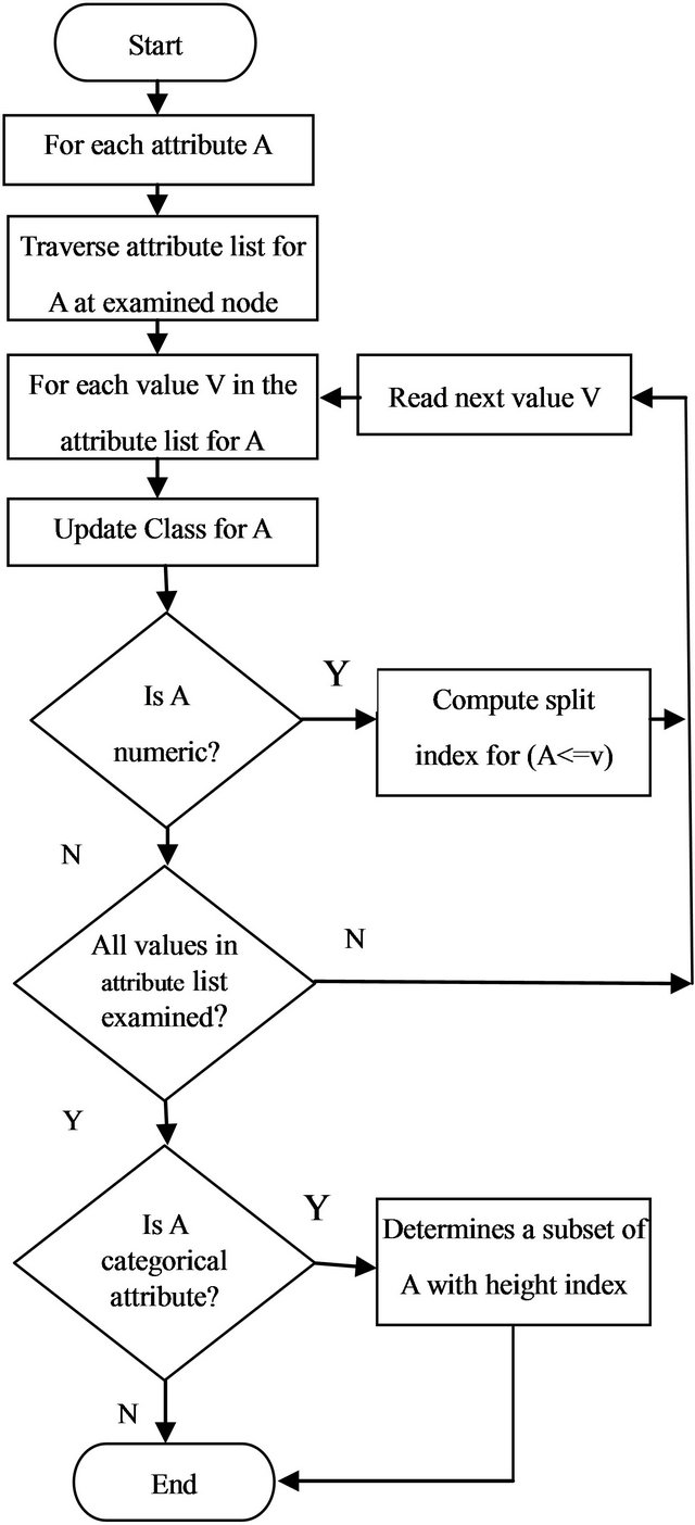
Figure 1. Flowchart of C4.5 decision tree algorithm.
The idea behind Naïve Bayes algorithm is the posterior probability of a data instance ti in a class cj of the data model.
The posterior probability P(ti|cj) is the possibility of that ti can be labeled cj. P(ti|cj) can be calculated by multiplying all probabilities of all attributes of the data instance in the data model:
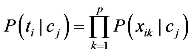
with p denoted as the number of attributes in each data instance. The posterior probability is calculated for all classes, and the class with the highest probability will be the instance’s label. The flowchart of this algorithm is presented in Figure 2.
Classification (also known as classification trees or decision trees) is a data mining algorithm that creates a step-by-step guide for how to determine the output of a new data instance. The tree it creates is exactly that: a tree whereby each node in the tree represents a spot where a decision must be made based on the input, and we move to the next node and the next until we reach a leaf that tells you the predicted output.
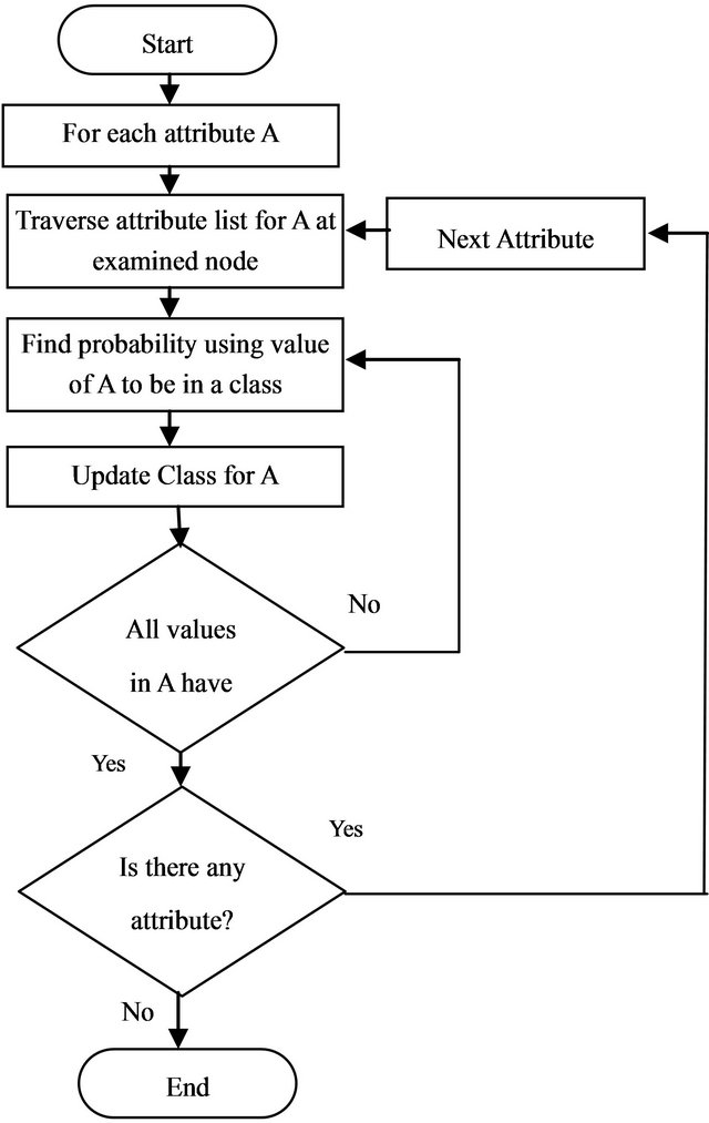
Figure 2. Flowchart of Naïve Bayes decision tree algorithm.
The classification tree literally creates a tree with branches, nodes, and leaves that lets us take an unknown data point and move down the tree, applying the attributes of the data point to the tree until a leaf is reached and the unknown output of the data point can be determined. We learned that in order to create a good classification tree model, we need to have an existing data set with known output from which we can build our model. We also divide our data set into two parts: a training set, which is used to create the model, and a test set, which is used to verify that the model is accurate and not over fitted.
The dataset used in this research is related with direct marketing campaigns of a Portuguese banking institution. The marketing is done by phone calls. The classification goal is to predict if the client will subscribe a term deposit. There are total 45,211 records in dataset. Each record has 17 attributes including the last attribute defines the class label of the record, whether the customer subscribe to term deposit or not. More details about those data and their attributes could be found in [12]. We divide data into two parts. One is for training and another is for testing. The training data set contains whole data (45,211 records). The testing data set contains 10% of whole data (4521 records), randomly selected from the whole data set.
Using C4.5, after the training the correctly classified instances are 42,554 which are 94.1231% and incorrectly classified instances are 2657 which is 5.8769%. So we can say that the training is good. And after the testing the correctly classified instances are 4248 which is 93.9615% and the incorrectly classified instances are 273 which are 6.0385%. So we can say that the model can classify accurately. Comparing the “Correctly Classified Instances” from this test set (93.96 percent) with the “Correctly Classified Instances” from the training set (94.12 percent), we see that the accuracy of the model is close, which indicates that the model is strong.
Using Naïve Bayes, after the training the correctly classified instances are 39,811 which are 88.056% and incorrectly classified instances are 5400 which is 11.944%. So we can say that the training is good. And after the testing the correctly classified instances are 3966 which is 87.724% and the incorrectly classified instances are 555 which are 12.276%. So we can say that the model can also classify accurately.
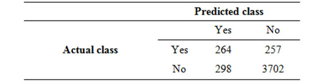
A confusion matrix contains information about actual and predicted classifications done by a classification system. Performance of such systems is commonly evaluated using the data in the matrix [13]. The following tables (Tables 1 and 2) show the confusion matrix for a two class classifier.
We have used decision tree to analysis result and bring out the goal of our work. A decision tree is a classifier in
Table 1. Confusion matrix using C4.5 algorithm.
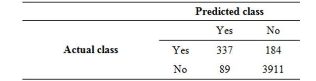
Table 2. Confusion matrix using Naïve Bayes algorithm.
the form of a tree structure, where each node is either:
1) A leaf node-indicates the value of the target attribute (class) of examples, or 2) A decision node-specifies some test to be carried out on a single attribute-value, with one branch and subtree for each possible outcome of the test. A decision tree can be used to classify an example by starting at the root of the tree and moving through it until a leaf node, which provides the classification of the instance. Decision tree induction is a typical inductive approach to learn knowledge on classification. The key requirements to do mining with decision trees are attribute-value description:
Object or case must be expressible in terms of a fixed collection of properties or attributes. This means that we need to discretize continuous attributes, or this must have been provided in the algorithm.
A. Predefined classes (target attribute values): The categories to which examples are to be assigned must have been established beforehand (supervised data).
B. Discrete classes: A case does or does not belong to a particular class, and there must be more cases than classes.
C. Sufficient data: Usually hundreds or even thousands of training cases.
The estimation criterion in the decision tree algorithm is the selection of an attribute to test at each decision node in the tree. The goal is to select the attribute that is most useful for classifying examples. A good quantitative measure of the worth of an attribute is a statistical property called information gain that measures how well a given attribute separates the training examples according to their target classification. This measure is used to select among the candidate attributes at each step while growing the tree.
Knowledge Discovery in Databases (KDD) [3,6,13,14] is an active area of research that resolves the complexity mentioned above. Knowledge discovery in databases is the effort to understand, analyze, and eventually make use of the huge volume of data available. Through the extraction of knowledge in databases, large databases will serve as a rich, reliable source for knowledge generation. It combines many algorithms and techniques used in Artificial Intelligence, statistics, databases, machine learning, etc. KDD is the process of extracting previously unknown, not obvious, new, and interesting information from huge amount of data. KDD is the extraction of interesting patterns in large database. It has been recognized that a discovery system can generate a plenty of patterns which may be no interest. This is one of the central problems in the field of knowledge discovery in the development of good measures of interestingness of the discovered patterns. In the next part we have used some data from database to extract actionable knowledge.
4. Result Analysis
It is very difficult to make a judgment that a classification algorithm is better than another because it may work well in a certain data environment, but worse in others. Evaluation on performance of a classification algorithm is usually on its accuracy. However, other factors, such as computational time or space are also considered to have a full picture of each algorithm.
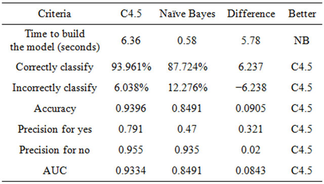
We have used a set of training data and then test. Both the training and testing applied for C4.5 and Naïve Bayes algorithm using WEKA. Table 3 presents the performance of the algorithms on testing data set. We can predict the better model from the following information. Each of the performance metric is described in detail next.
4.1. Time to Build the Model
If a dataset contains millions of training data with many attributes, and the number of training loops on the set is high, the network will take very long time on a typical computer to arrive with a model. The other algorithms run very fast not only in any data environment. However, the more data and the longer time a neural network is train with, the better result it will produce. Here C4.5 takes more time to build the model.
Table 3. Evaluation of the two models.
4.2. Correctly and Incorrectly Classify
Correctly classify ratio is important to show the performance of a model. The model will be stronger if it classifies records more correctly.
4.3. Accuracy
The accuracy is the proportion of the total number of predictions that were correct. The accuracy of both the model is high. C4.5 is better than Naïve Bayes. The database used here is noise free. On the other hand the database is large. So accuracy is high. Generally for machine learning approach much collection of data brings the more accuracy. Figure 3 shows the True Positive (TP) rate for two classification algorithms where Figure 4 depicts the accuracy of those two models.
4.4. AUC
Areas under the ROC curve (AUCs), while classification accuracy is maintained in high values and rule set sizes are substantially reduced. Also, the method compared adequately against other good probability estimators. Receiver Operating Characteristic (ROC) graphs is another way besides confusion matrices to examine the performance of classifiers. A ROC graph is a plot with the false positive rate on the X axis and the true positive rate on the Y axis. The point (0, 1) is the perfect classifier: it classifies all positive cases and negative cases correctly. It is (0, 1) because the false positive rate is 0 (none), and the true positive rate is 1 (all). The point (0, 0) represents a classifier that predicts all cases to be negative, while the point (1, 1) corresponds to a classifier that predicts every case to be positive. Point (1, 0) is the classifier that is incorrect for all classifications.
If we see the ROC curve both for the classes in Figures 5 and 6, yes and no, then it seems to be closer to y axis (true positive). ROC of yes class is closer than of
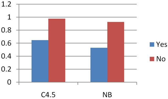
Figure 3. True positive rate.
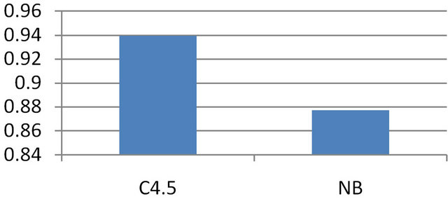
Figure 4. Accuracy of two models.
class no. It is characteristics of good classification. On the other hand the AUC are for the both class is 0.9334. The area under the ROC curve (AUC) is a method of measuring the performance of the ROC curve If AUC is 1 then the prediction is perfect. If it is 0.5 then the prediction is random. For Naïve Bayes classification we get lower ROC and AUC as well. This is depicted in Figures 7 and 8 for “no” and “yes” class respectively.
4.5. Precision
The precision is the proportion of the predicted positive cases that were correct. Figure 9 depicts the precision of those two models.
Figures 10 and 11 show the classify error for both algorithms.
To the right of the plot area there are series of horizontal strips. Each strip represents an attribute, and the dots within it show the distribution values of the attribute. The following Figures 10 and 11 show strips of 16 attributes and 2 strips for the two classes (yes and no). The both plots show the results of classification. Correctly classified instances are represented as crosses, incorrectly classified one is represented as squares. There are similarities between two figures (C4.5 and Naïve Bayes). The left lower corner and upper right corner shows cross indicating correctly classified. The upper left corner and lower right corner of the graph, there are two squares in this corner. The squares represent incorrectly classified instances.
The ratio for the correctly and incorrectly classify are satisfactory. Both the model strongly classified the expected class.
As can be seen both the algorithm have comparable performance. Though the Naïve Bayes takes less time than C4.5 to build the model but other criteria proved that C4.5 is better. So we can take C4.5 for more accuracy and prediction of data.
4.6. Knowledge Discovery and Actionable Knowledge
Preprocessing the input data set for a knowledge discovery goal using a data mining approach usually consumes the biggest portion of the effort devoted in the entire work. Actionable rules are applied on data mining to extract unknown, hidden and required pattern. It is the implementation of data mining. We have used C4.5 and Naïve Bayes algorithm to predict the actionable knowledge. Actionability is the most important measure among all the subjectivity measures. It is effective in decision making and finding patterns. There is an automated information technology that can capture and analyze not just information but actionable information. One of the data mining issues is to make the mined patterns action-
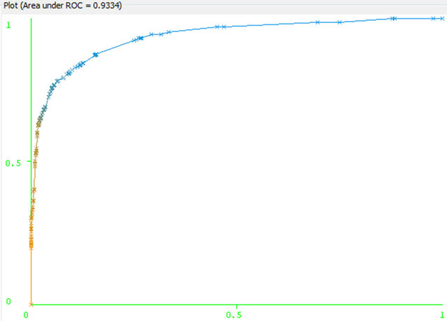
Figure 5. C4.5 ROC curve for class: Yes.
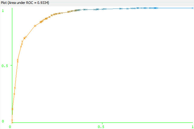
Figure 6. C4.5 ROC curve for class: No.

Figure 7. Naïve Bayes ROC for yes class.
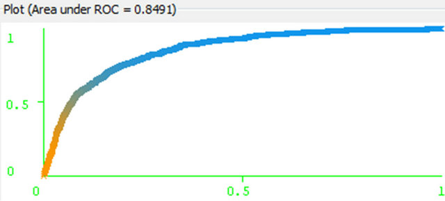
Figure 8. Naïve Bayes ROC for no class.
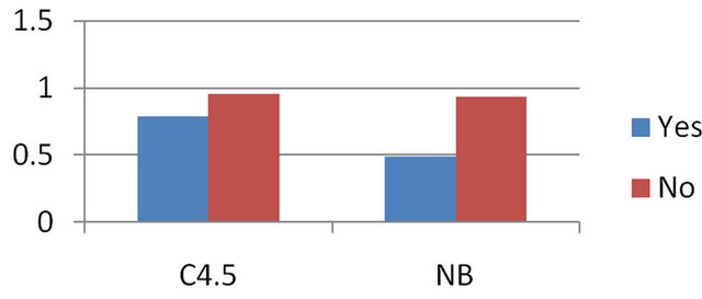
Figure 9. Precision for the class Yes and No from both the algorithms.
able [8,14,15]. There are both numeric and nominal data in the data source. If we analyze the Naïve Bayes run information we can predict actionable knowledge. The run information part contains general information about the scheme used.
Generally a customer will subscribe a term deposit if1) His/her job type is management or technician or blue-color or admin but management has the high priority.
2) If he/she is married.
3) Education is secondary or tertiary.
4) Has no credit in default.
5) Average yearly balance is around EUR1804.3002.
6) Has no housing loan.
7) Has no personal loan.
8) Contact communication type is cellular.
9) Last contact month is (priority basis) May or August or July or April.
10) Last contact duration is around 537.2908 second.
11) Number of contact to him/her is around 2.4345 times.
12) Around 68.3406 days passed after the last contact.
13) Number of contact performed is around 0.8449.
14) The outcome of previous marketing campaign is unknown.
If a customer data satisfy the above information then we can predict that there is a high probability of the customer to subscribe a term deposit.
If we analyze the C4.5 decision tree then we found data those rules has a co-relation with the Naïve Bayes algorithm. C4.5 shows the evaluation with every particular data but Naïve Bayes’s evaluate with a data of its correspondence group.
For the best C4.5 tree, the rules are obtained were in summary:
1) Contact communication type is cellular.
2) Last contact duration is >130.
3) Education is tertiary or secondary.
4) No housing loan.
5) 3 days ago of contact.
6) Yearly balance is >103.
7) Last contact month of the year is July or August or October.
8) Job type is management or technician.
Based on the above decision marketing department can decide a group of customer for marketing investment. After evaluating model one with another increase the confidence. Institutional sensitive issues depend on marketing strategy. So it is also a cost effective solution for targeting a customer and campaign. This has important implications for business behavior.
Novel algorithm is used here to extract actionable knowledge. It works post processing technique to mine actionable knowledge from decision tree. To bring the actionable knowledge to a customer relation management (CRM) decision tree is created. There are probabilities of a customer to change his/her status from one state to another.
In [4], Yang et al. propose novel algorithms for post processing decision trees to obtain actions that are associated with attribute-value changes, in order to maximize the profit-based objective functions. This allows a large number of candidate actions to be considered, complicating the computation.
The overall process of the algorithm can be briefly described in the following four steps:
1) Import customer data with data collection, data cleaning, data preprocessing, and so on.
2) Build customer profiles using an improved decision tree learning algorithm from the training data. In this case, a decision tree is built from the training data to predict if a customer is in the desired status or not. One improvement in the decision tree building is to use the area under the curve (AUC) of the ROC curve, to evaluate probability estimation (instead of the accuracy).
3) Search for optimal actions for each customer. This is a key component of the data mining system Proactive
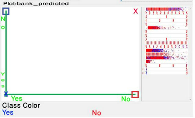
Figure 10. Visual classification error of C4.5.
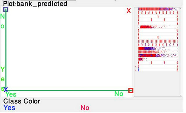
Figure 11. Visual classification error of Naïve Bayes.
Solution.
4) Produce reports for domain experts to review the actions and selectively deploy the actions.
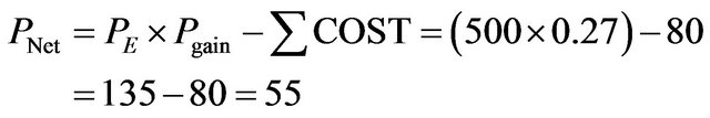
The leaf node search algorithm searches for optimal actions to transfer each leaf node to another leaf node with a higher probability of being in a more desirable class. We also use their technique in this research. After building the decision tree we can calculate the net profit.

PNet: Net profit;
PE: Total profit of the customer in the desired status;
Pgain: The probability gain;
COST: The cost of each action involved.
Algorithm leaf node search 1) For each customer x, do 2) Let S be the source leaf node in which x falls into;
3) Let D be a destination leaf node for x the maximum net profit PNet;
4) Output (S, D, PNet);
Using data mining tools and techniques, we summarized a group customer with specific characteristic. This group of customer has high probability to be a term depositor. There will be some decision tree where customer falls in a leaf node. Target is that move the customer from one node to another to be a term depositor. Then bank will take steps to chance the characteristic so that they can fall into a desired node and they will be a term depositor. Steps may be some offer for the customer or making some term flexible for customer. Facility is that not to target or campaign for mass amount of customer, only a group of customer there will be high probability to be a term depositor. It will decrease yearly cost and maximize the profit.
Let us explore with some examplesExample 1 Using data mining we have found that customer who has no housing loan has high probability to be a term depositor. Bank’s task is to declare offer which encourage customer to finish the loan. The algorithm works as the following.
The bank has observed that many customers are fallen in node A and node B as depicted in Figure 12. Our target is to change customer’s characteristic by which they fall into leaf node B from A. Then the probability gain is 27% (63% − 36%). Assume that cost of changes from A to B is $80 (given by the bank). If the bank can make a total profit of $500 then the probability gain (27%) is converted into $135 (5000 × 0.27). therefore the net profit would be $55 (135 − 80).
So bank can now promote finish the loan or offer to finish loan in certain terms and condition.
Example 2 Another interesting example may be the customer’s marital status which is presented in Figure 13. Data mining shows that married person are interested for term deposit.
Bank’s target is to take the customer from B or A in to A. or can take from B to C. The first one is better. If a customer fall in C then the algorithm search through all the leaf in the decision tree to see the height net profit.
1) Focusing on leaf A. The probability of gain is 16% (52% − 36%) if the customer falls into A. action need to change marital status from single to married. Assume that cost of such change is $100 (given by bank). If the bank can make a total profit of $1000 from the customer, then this probability gain (16%) is converted into $160 (1000 × 0.16) of the expected gross profit. Therefore, the net profit would be $60 (160 − 100).
2) Similarly focusing on leaf B. It has a lower probability of being loyal, so the net profit must be negative, and we can safely skip.
So the node with maximal net profit is A.
Notice that actions suggested for customer status change imply only correlations (not causality) between customer features and status. Like other data mining systems, the results discovered (actions here) should be reviewed by domain experts before deployment. The algorithm for searching the best actions can thus be described as follows: for each customer, search every leaf node in the decision tree to find the one with the maximum net profit.
4.7. Profit Optimal Decision Tree and SBP
Decision trees are produced by algorithms that identify various ways of splitting a data set into branch like segments [4,5,10]. These segments form an inverted decision tree that originates with a root node at the top of the tree. The object of analysis is reflected in this root node as a simple, one-dimensional display in the decision tree
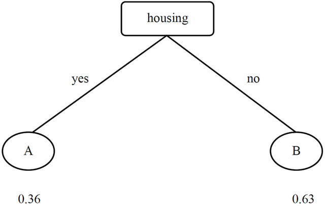
Figure 12. Split based on housing.
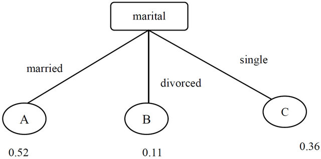
Figure 13. Split based on marital status.
interface. In general we build tree by choosing split. Generally we follow the steps like:
Try different partitions using different attributes and splits to break the training examples into different subsets.
Rank the splits (by purity). Choose the best split.
For each node obtained by splitting, repeat until no more good splits are possible.
In this way we build tree that is a good tree but it could be more profitable if we split the tree in different way. We get profit from this way and so called profit optimal decision tree.
Profit-optimal partition is a different tree structure entirly. Sequential decision problems arise in many areas, including communication net works, artificial intelligence and computer science. If we use sequential binary programming (SBP) in decision tree then it will be a profit optimal model. Difference between it and previous is that split the tree in different way. It works as the followings:
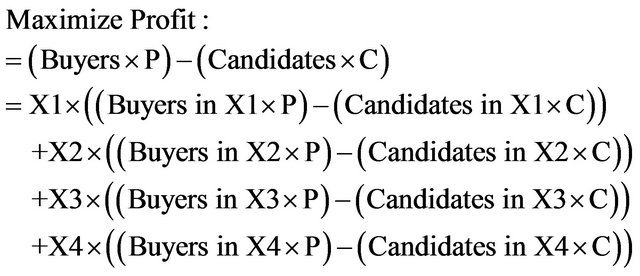
For each level of the tree, starting at the root, solve the following binary integer program:
Decision Variables:
Xi = Use partition i or not (binary)
For each attribute, try different cut-off values (partitions).
For example:
X1 = Partition is “Age > 0”
X2 = Partition is “Age > 20”
X3 = Partition is “Age > 40”
X4 = Partition is “Age > 60”
Constraints:
Xi are binary Exactly one partition is chosen at a time: SXi = 1 Profit per customer = P Cost per customer = C Objective function:
Previously we have mentioned that generally person who are married have more chance to be a term depositor (customer). Profit-optimal partition is a different tree structure entirely. Traditional decision tree splits the data in married and other as the following (Figure 14).
4.8. Splitting According to Married
Total married person is 2797 where 277 are customer and 2520 are not.
Assume:
Cost of contacting candidate = R1 Profit from customer = R10 Then,
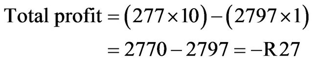
That means it is loss project if contact to only married person.
4.9. Splitting According to Single
Total single person is 1196 where 167 are customer and 1029 are not.
Then,
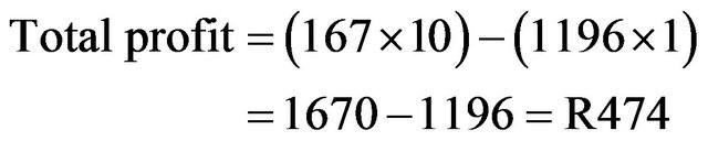
In this case profit ratio is higher than above.
4.10. Splitting According to Divorced
Total single person is 528 where 77 are customer and 451 are not.
Then,
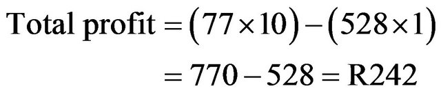
In this case profit ratio is higher than married person but lower than single.
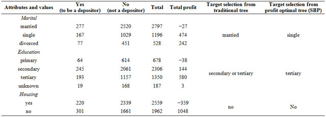
Though there is a high probability of married person to be a term depositor but profit is low. Table 4 presents output of using profit optimal decision tree. It is applied only marital, education and housing attributes. To calculate all the value and comparing we have used Microsoft excel. Countifs function is used to calculate cross checking value.
5. Conclusion
Before the application of actionable algorithm we need to analyze the data using some data mining tools and techniques. Evaluation and comparison of such techniques are also important to take close to satisfactory decision.
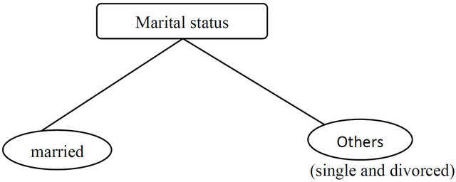
Figure 14. Another example of split to marital status.
Table 4. Output of using profit optimal decision tree.
We have used two popular data mining algorithm C4.5 and Naïve Bays to summarize data for selecting a group of customer. Then a novel algorithm [4-7] is used to extract actionable knowledge. This algorithm processes decision tree and obtain actions that are associated with attribute-value changes of the clients from one status (not a depositor) to another (depositor).
REFERENCES
- C. X. Ling and C. Li, “Data Mining for Direct Marketing: Problems and Solutions,” Proceedings of International Conference on Knowledge Discovery from Data (KDD 98), New York City, 27-31 August 1998, pp. 73-79.
- G. Dimitoglou, J. A. Adams and C. M. Jim, “Comparison of the C4.5 and a Naïve Bayes Classifier for the Prediction of Lung Cancer Survivability,” Journal of Computing, Vol. 4, No. 2, 2012, pp. 1-9.
- P. S. Vadivu and V. K. David, “Enhancing and Deriving Actionable Knowledge from Decision Trees,” International Journal of Computer Science and Information Security (IJCSIS), Vol. 8, No. 9, 2010, pp. 230-236.
- M. Alam and S. A. Alam, “Actionable Knowledge Mining from Improved Post Processing Decision Trees,” International Conference on Computing and Control Engineering (ICCCE 2012), Chennai, 2012, pp. 1-8.
- R. A. Patil, P. G. Ahire, P. D. Patil, Avinash and L. Golande, “Decision Tree Post Processing for Extraction of Actionable Knowledge,” International Journal of Engineering and Innovative Technology (IJEIT), Vol. 2, No. 1, 2012, pp. 152-155.
- Q. Yang, J. Yin, C. Ling and R. Pan, “Extracting Actionable Knowledge from Decision Trees,” IEEE Transaction on Knowledge and Data Engineering, Vol. 19, No. 1, 2007, pp. 43-56.
- Q. Yang, J. Yin, C. X. Ling and T. Chen, “Post Processing Decision Trees to Extract Actionable Knowledge,” Proceedings of the Third IEEE International Conference on Data Mining (ICDM’03), 19-22 November 2003, Florida, pp. 685-688. doi:10.1109/ICDM.2003.1251008
- Z. He, X. Xu and S. Deng, “Data Mining for Actionable Knowledge: A Survey,” ArXiv Computer Science e-Prints, 2005.
- J. Huang, J. Lu and C. X. Ling, “Comparing Naïve Bayes, Decision Trees, and SVM with AUC and Accuracy,” Proceedings of Third IEEE International Conference on Data Mining (ICDM 2003), 19-22 November 2003, pp. 553-556. doi:10.1109/ICDM.2003.1250975
- A. Abrahams, F. Hathout, A. Staubli and B. Padmanabhan, “Profit-Optimal Model and Target Size Selection with Variable Marginal Costs,” 2013. http://www.cl.cam.ac.uk/research/srg/opera/publications/papers/abrahams-wharton-working-paper-feb04.pdf
- Weka Data Mining Tool. http://www.cs.waikato.ac.nz/ml/weka/
- UCI Machine Repository Data. http://archive.ics.uci.edu/ml/datasets/Bank+Marketing
- H. Kaur, “Actionable Rules: Issues and New Directions,” World Academy of Science, Engineering and Technology, Vol. 5, 2005, pp. 61-64.
- T. Goan and S. Henke, “From Data to Actionable Knowledge: Applying Data Mining to the Problem of Intrusion Detection,” Proceedings of International Conference on Artificial Intelligence (IC-AI’2000), Las Vegas. http://citeseerx.ist.psu.edu/viewdoc/summary?doi=10.1.1.118.9792
- R. D’Souza, M. Krasnodebski and A. Abrahams, “Implementation Study: Using Decision Tree Induction to Discover Profitable Locations to Sell Pet Insurance for a Startup Company,” Journal of Database Marketing & Customer Strategy Management, Vol. 14, No. 4, 2007, pp. 281-288. doi:10.1057/palgrave.dbm.3250059