Journal of Biomedical Science and Engineering
Vol.7 No.5(2014), Article ID:45165,11 pages DOI:10.4236/jbise.2014.75032
A Finite Element Model for Recognizing Breast Cancer
Ashraf Ali Wahba1, Nagat Mansour Mohammed Khalifa2, Ahmed Farag Seddik1, Mohammed Ibrahim El-Adawy1
1Faculty of Engineering, Biomedical Engineering Department, Helwan University, Cairo, Egypt
2Radio-Diagnosis National Cancer Institute, Cairo University, Cairo, Egypt
Email: ashraf_wahba@h-eng.helwan.edu.eg, nagatmansour@gmail.com, ahmed_sadik@h-eng.helwan.edu.eg, mohamed@eladawy.com
Copyright © 2014 by authors and Scientific Research Publishing Inc.
This work is licensed under the Creative Commons Attribution International License (CC BY).
http://creativecommons.org/licenses/by/4.0/


Received 7 March 2014; revised 10 April 2014; accepted 18 April 2014
ABSTRACT
Breast cancer recognition is an important issue in elastography diagnostic imaging. Breast tumor biopsy has been for many years the reference procedure to assess histological definition for breast diseases. But biopsy measurement is an invasive method besides it takes larger time. So, fast and improved methods are needed. Using elastography technology, a digital image correlation technique can be used to calculate the displacement of breast tissue after it has suffered a compression force. This displacement is related to tissue stiffness, and breast cancer can be classified into benign or malignant according to that displacement. The value of compression force affects the displacement of tissue, and then affects the results of the breast cancer recognition. Finite element method was being used to simulate a model for the breast cancer as a phantom to be used in measurements and study of breast cancer diagnosis. The breast cancer using this phantom can be recognized within a short time. The proposed work succeeded in recognizing breast tumor phantom by an average correct recognition ratio CRR of about 94.25% on a simulation environment. The strain ratio SR for benign and malignant models is also computed. The result of the simulated breast tumor model is compared with real data of 10 lesion cases (6 benign and 4 malignant). The coefficient of variation CV between the simulated SR and the SR using real data reaches to about 5% for benign lesions and 4.78% for malignant lesions. The results of CRR and CV in this proposed work assure that the proposed breast cancer model using finite element modeling is a robust technique for breast tumor simulation where the behavior of real data of breast cancer can be predicted.
Keywords:Breast Cancer, Digital Image Correlation, Ultrasound Elastography, Strain Analysis, Breast Cancer Diagnosis

1. Introduction
This paper introduces a simulation algorithm for breast cancer recognition. The breast is made up of lobes and ducts. Each breast has 15 to 20 sections called lobes which have many smaller sections called lobules. Lobules end in dozens of tiny bulbs that can make milk. The lobes, lobules, and bulbs are linked by thin tubes called ducts. Each breast also has blood vessels and lymph vessels. The lymph vessels carry colorless fluid called lymph. Lymph vessels lead to organs called lymph nodes. Lymph nodes are small bean-shaped structures that are found throughout the body. They filter substances in a fluid that called lymph and help fight infection and disease. Clusters of lymph nodes are found near the breast in the axilla (under the arm), above the collarbone, and in the chest. The most common type of breast cancer is ductal carcinoma, which begins in the cells of the ducts. Cancer that begins in the lobes or lobules is called lobular carcinoma. Inflammatory breast cancer is an uncommon type of breast cancer in which the breast is warm, red, and swollen. Breast cancer spreads in the body through three ways. They are blood, tissue, and lymph nodes [1] .
The early detection of breast cancer is an important issue in breast cancer treatment and curing [2] [3] . Elastography techniques are widely used in breast cancer diagnosing [4] -[7] , especially the colored elastography techniques that assign a certain color to each degree of stiffness of breast tumor [8] . Also, elastography can be used in breast lesion characterization [9] -[10] in order to construct a classifier used for breast tumor staging [11] . Diagnostic ultrasound imaging [12] [13] using elastic properties of breast lesion [14] [15] is used to get a high percentage of correct diagnosis for breast tumor in order to decide the suitable steps and the best treatment for this invasive cancer. In this proposed work an algorithm is being illustrated to recognize breast cancer which is simulated by a finite element method and improved this recognition algorithm by using a simulated reference material as an impedance matching material. This matching material is being put between the compression force surface and the simulated breast tissue. These simulated results on the breast tumor model can be evaluated using real data and real reference material as follows in the proposed work method.
2. Materials and Method
The aim of this work is to build a finite element model FEM representing a compression elastography technique. The proposed recognition algorithm is shown in Figure 1. This algorithm composes of the following five basic steps [16] :
1) Initialization step.
2) Applying of compression forces.
3) Get the FEM for breast before and after compression.
4) Correlation of the deformed model resulted from the FEM.
5) Breast cancer recognition.
2.1. Initialization Step
The ultrasound of breast was discussed in various works [7] . Many previous works concentrated on studying breast cancer through biopsy measurements which is the main reference measurements in breast cancer diagnosis [17] , and other works focused on ultrasound imaging of breast cancer [7] [13] . Phantoms can be used to mimic the soft tissue and other parts in human body, to be tested using ultrasound imaging. These phantoms used to assess the accuracy of using ultrasound imaging in tumor diagnosis [18] [19] . In this proposed work, an elastography technique based on a multi-compression force is being used. It is assumed that breast tumor stiffness values were calculated before from biopsy measurements, and these values will be used as references when recognize breast cancer from elastography images.
2.2. Simulated Benign and Malignant Breast Images
Finite element method FEM using ABAQUS software is used to simulate breast models [20] -[22] . Finite element model of breast cancer is represented as shown in Figure 2. A reference material with stiffness of Er = 5 KPa is used to get impedance matching and good ultrasound wave transmission performance. We put this reference material between the soft tissue and the applied force surface in order to use it in stiffness calculation as in Section 2.5. In ABAQUS software, the stiffness of the simulated materials is assumed to be 5 KPa, 20.5 KPa, and 168 KPa for the reference material which was proposed to be the silicon rubber, benign tissue, and malignant tissue respectively [17] .
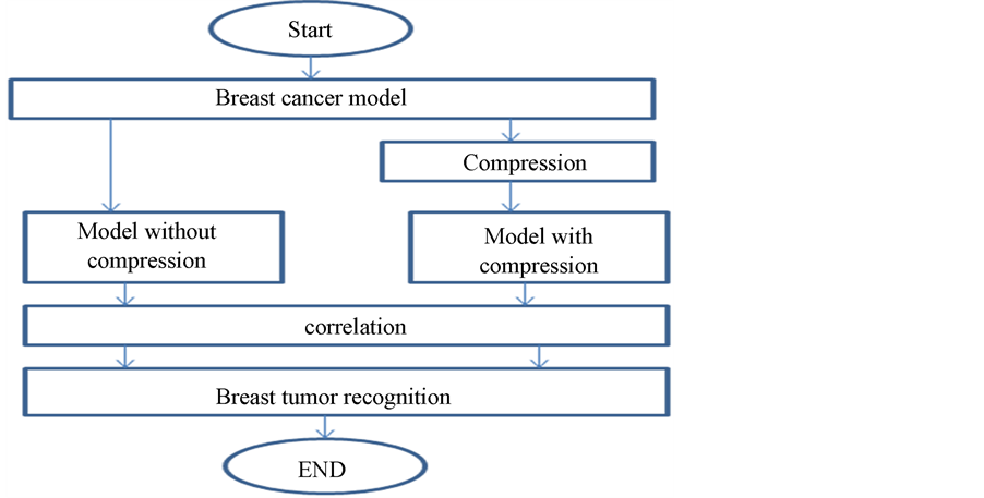
Figure 1. Block diagram of breast cancer recognition algorithm.
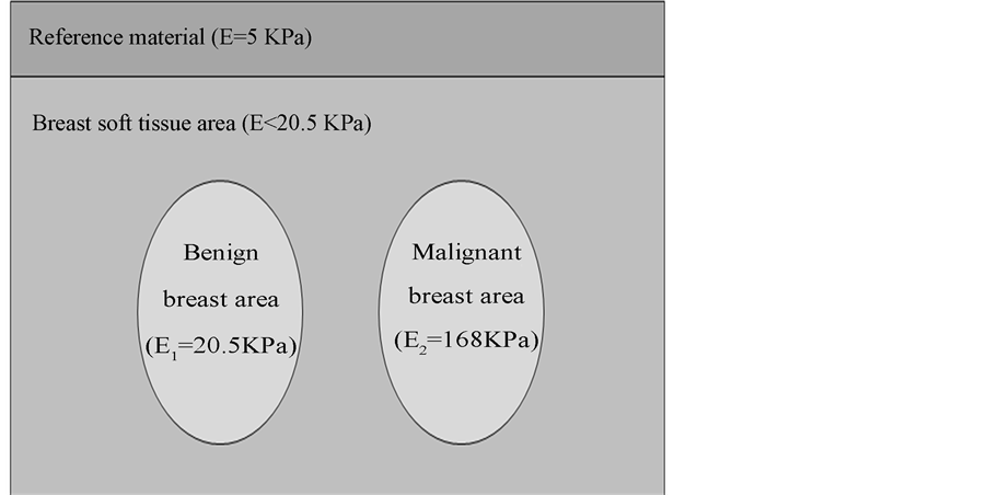
Figure 2. Benign and malignant breast models using finite element method.
2.3. Application of Compression Forces
In FEM, a certain compression force was applied on the proposed model in Figure 2. Model before and after compression, will be taken to be correlated using the digital image correlation technique as described in the next section.
2.4. Image Correlation
Digital image processing is a main tool to describe image details and image features [23] [24] . To calculate the displacement that the pixels of the deformed image move when suffered to a compression force, a digital image correlation technique may be used. The steps of using the two dimension (2D) digital image correlation are as follows:
1) Input to the correlation function [25] -[29] the deformed (compressed) and un-deformed (un-compressed) images for correlation, and assign the first image (un-deformed or un-compressed) as a reference image for correlation.
2) The correlation function is used to match a subset from the reference image to another in the second deformed image and can be written as follows in Equation (1) [16] [28] .
 (1)
(1)
where F(x, y) and G(x*, y*) represent the gray levels within the subset of the un-deformed and deformed images respectively. R is the magnitude of intensity value difference. Also, (x, y) and (x*, y*) are the coordinates of a point on the subset before and after deformation respectively. The symbol of the summation represents the sum of the values within the subset. The coordinate (x*, y*) after deformation relates to the coordinate (x, y) before deformation, therefore, displacement components are obtained by searching the best set of the coordinates after deformation (x*, y*) which minimize R(x, y, x*, y*).
3) Make a grid on the reference image for the part needed to be correlated. The grid will contain a number of N rasters Mn, where n varies from 0 to N ‒ 1, and each raster Mn represents number of pixels of the FEM of breast image. Assuming that the motion is in one direction only x, then, the position of rasters will be in x direction only and denoted by grid_x.
4) Run the correlation function to the previous grid. The function will give the new position of the grid rasters on the compressed image in x direction, which is denoted by validx.
5) The displacement for each grid point ∆Lx in x direction (the direction of the applied force) can be calculated as follows in Equation (2) [16] :
 (2)
(2)
2.5. Breast Cancer Recognition Using FEM
Breast tumor can be recognized according to the displacement ∆Lx calculated in Equation (2). Hooke’s law specifies that the force affecting material is directly proportional to the displacement occurred on each part of this material as follows in Equation (3) [16] [30] -[33] .

where: F is the applied force; K is a constant depends on the elasticity or the stiffness of the material, and X is the displacement. If the force F is fixed at a constant value, then the displacement will depend only on the elasticity of the material which changes from material to another. The relation between the displacement ∆Lx and the stiffness E is as follows in Equation (4) [16] :
 (4)
(4)
where A is the cross section area of the material under stress, L is the initial length, and ∆Lx is the displacement.
If L, A, and F are assumed to be constants, then from Equation (4) we can see that the stiffness E is inversely proportional to the displacement ∆Lx as follows in Equation (5) [16] ;
 (5)
(5)
To eleminate the need for a proportionality constant we can write the stiffness of any two materials as follows in Equation (6) [16] ;
 (6)
(6)
The proposed work uses different forces for compression, and with each force the displacement ∆Lxn of each raster Mn will be calculated through the correlation function. ∆Lxn is assumed to be the displacement of the checked raster. ∆Lxr is assumed to be the displacement of the reference raster that has been located in the reference material which has a stiffness value of Er = 5 (KPa). Also, E1 and E2 are assumed to be the stiffness values of benign and malignant breast tissue respectively. According to the proposed work, the checked rasters n can be classified according to Equations (7) to (10) [16] to be one of the following materials; reference material, soft tissue, benign breast tumor with stiffness of E1, or malignant breast tumor with stiffness of E2.
 (7)
(7)
 (8)
(8)
 (9)
(9)
 (10)
(10)
After correlation, rasters will be classified as soft, benign, or malignant tissues. Results of this classification will be compared with the original assumed tissues. Different compression forces will be applied and an average classification result will be calculated from which we can find the correct recognition ratio, CRR, as follows in Equation (11):
 (11)
(11)
2.6. Strain Ratio for Simulated Breast Lesions
Tissue strain analysis is important for tissue stiffness characterization [34] and can be studied using ultrasound elastography [35] . Using Equation (2), the strain for each grid point Sx in x direction in the proposed model can be calculated as follows in Equation (12):
 (12)
(12)
Also, the average strain Ssav and Slav for the breast soft tissue and breast lesion respectively can be calculated as follows in Equations (13) and (14) respectively:
 (13)
(13)
 (14)
(14)
where Ns and Nl are the number of grid points in breast soft tissue and breast lesion respectively. The strain ratio SR for the breast soft tissue and breast lesion can be calculated as follows in Equation (15):
 (15)
(15)
This value of the SR calculated from the proposed finite element model will be compared with the SR value obtained from real images of breast cancer patients in the next section.
2.7. Strain Ratio for Real Breast Lesions
Real images were taken at National Cancer Institute in Cairo, Egypt using HITACHI Sonograph on 10 lesions (6 benign and 4 malignant). The images are taken before and after compression using an acoustic matching material of silicon rubber which put between the ultrasound transducer and the patient breast tissue. This silicon rubber material has stiffness value of 5 KPa and an acoustic impedance of 1.56 MRayl [36] as shown in Figure 3.
The average strain and strain ratio obtained from the Sonograph will be needed to be compared with the values obtained from the finite element model.
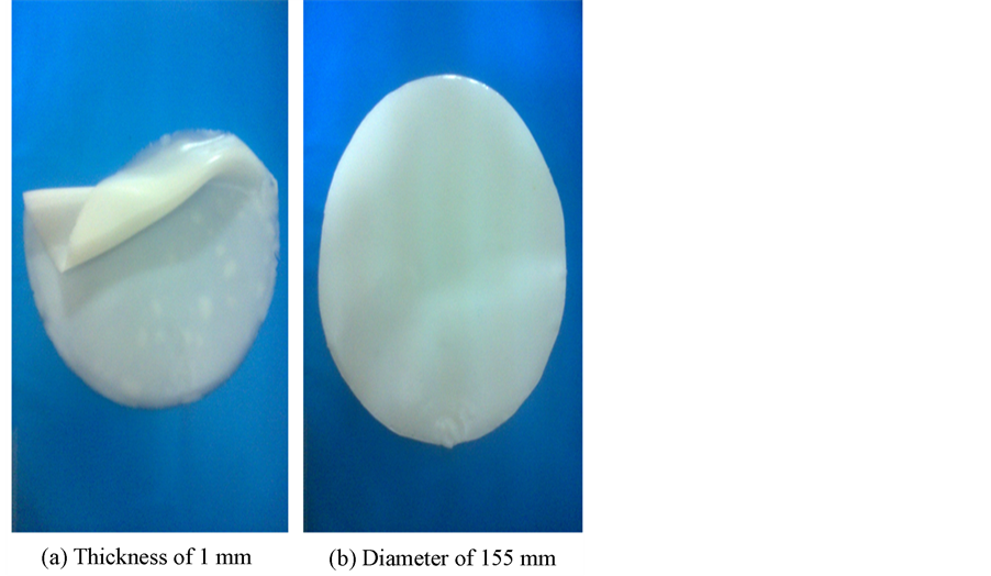
Figure 3. Silicon rubber of stiffness 5 KPa and acoustic impedance of 1.56 MRayl. (a) Shows the silicon rubber thickness; (b) Shows the silicon rubber diameter.
2.8. The Coefficient of Variation between the Simulated and Real Strain Ratio
The coefficient of variation, CV, between the simulated SR calculated using FEM and the real SR using real breast images which measured by HITASHI Sonograph can be calculated as follows in Equation (16):
 (16)
(16)
where σ is the standard deviation and can be calculated as follows in Equation (17):
 (17)
(17)
where N is the number of set points, Xi is the set of N points and µ is the mean value of the set points that can be calculated as follows in Equation (18):
 (18)
(18)
3. Results
3.1. Breast Cancer CRR Using FEM
To calculate the correctness of classification between different breast tumors we will follow these steps:
1) In the FEM domain we will consider set up of three areas, known as a reference material, soft tissue, and a known breast tumor area.
2) Consider 100 rasters distributed in each of the three areas where the position of each raster in these areas is known.
3) Apply a compression force in the direction from the reference material to the soft tissue to the tumor area. As results of the force, each raster will move certain displacement in the direction of the applied force depending on the material stiffness that contains this raster.
4) Use the correlation technique to recognize each raster’s new position after the force is applied.
5) From this new position of each raster, the displacement of this raster will be calculated.
6) Use Equations (6)-(10) to classify the material to be either reference, soft, benign, or malignant material.
7) According to the classification of each raster material we fill in Table 1, where from this table the correct recognition ratio CRR can be calculated for those 100 checked rasters affected by that specific force.
8) Changing the force and go to step (3) and repeat for 10 different values of the applied force, and in each case calculate CRR.
9) Calculate the average CRR on the 10 different forces.
10) Table 2 shows the average of the 10 tables where each one represents a certain compression force.
3.2. Strain Ratio for Breast Cancer Lesion Using FEM
The strain ratio for the simulated FEM breast lesion can be calculated using Equations (12), (13), and (14) as follows in Table 3.
3.3. Strain Ratio for Breast Cancer Lesion Using Real Breast Images
The strain ratio for the used 10 real breast lesions can be calculated using HITACHI Sonograph measurement. The strain ratio for the selected two cases of benign and malignant breast lesions is shown in Figure 4 and Figure 5 respectively.

Table 1. CRR for breast cancer using FEM model using one value of the applied force.
Table 2. Overall CRR result of applying 10 different values of the compression force with FEM model.
Table 3. The strain ratio of the breast lesion using FEM.
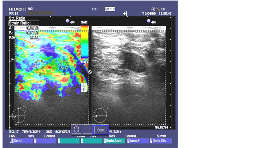
Figure 4. Benign breast lesion strain ratio image taken at National Cancer Institute in Cairo, Egypt by HITASHI Sonograph.
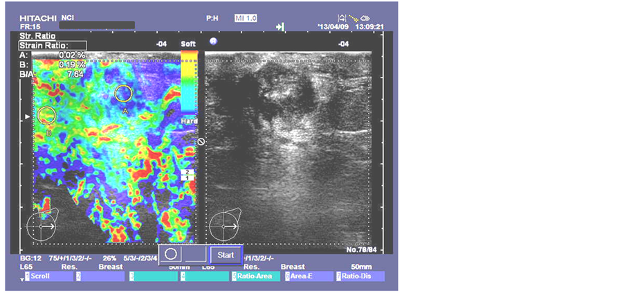
Figure 5. Malignant breast lesion strain ratio image taken at National Cancer Institute in Cairo, Egypt by HITASHI Sonograph.
The results of the strain ratio SR of the selected two cases of benign and malignant breast lesions that shown in Figure 4 and Figure 5 are as follows in Table 4.
The results of the average strain ratio SR for the 10 used breast lesions are as follows in Table 5.
3.4. The Coefficient of Variation CV between the Simulated and Real SR
The standard deviation σ between the simulated SR calculated using FEM and the real SR using real breast images is calculated using Equations (15) and (16) as follows in Table 6.
We notice that the strain ratio for benign is 0.8616 in simulated model and 0.954 for real data and this gives a CV of 5%, in this case the simulated model and real results are consistent. From Table 6 we can also notice the same for malignant lesions.
Table 4. The strain ratio of the selected two real breast lesion using HITASHI Sonograph.
Table 5. The average strain ratio of the 10 real breast lesion using HITASHI Sonograph.
Table 6. The coefficient of variation CV between the simulated and real SR.
4. Conclusion
This paper presents a finite element model for different breast tissues including soft, benign, and malignant tissues. This model can be considered as a software phantom that can be used to study breast cancer effects. Results from the model were compared with real data taken at National Cancer Institute in Cairo, Egypt by HITASHI sonograph. Results from the model and real data agreed to very good extent. As a metric for this agreement we calculated the coefficient of variation factor which was about 5% that indicates a good agreement.
References
- National Cancer Institute (2014) General Information about Breast Cancer—Stages of Breast Cancer. At the National Institutes of Health. http://www.cancer.gov/cancertopics/pdq/treatment/breast/Patient/page2
- NICE Clinical Guideline 80 (2009) Early and Locally Advanced Breast Cancer: Diagnosis and Treatment. Developed by the National Collaborating Centre for Cancer. National Institute for Health and Clinical Excellence, February.
- Khatib, O.M.N. and Modjtabai, A. (2006) Guidelines for the Early Detection and Screening of Breast Cancer. EMRO Technical Publications Series 30, World Health Organization.
- Treece, G., Lindop, J., Chen, L., Housden, J., Prager, R. and Gee, A. (2011) Real-Time Quasi-Static Ultrasound Elastography. Interface Focus, 1, 540-552. http://rsfs.royalsocietypublishing.org/content/1/4/540.full.html#related-urls
- Sette, M.M., Goethals, P., D’hooge, J., Van Brussel, H. and Vander Sloten, J. (2011) Algorithms for Ultrasound Elastography: A Survey. Computer Methods in Biomechanics and Biomedical Engineering, 14, 283-292. http://dx.doi.org/10.1080/10255841003766837
- Oelze, M.L., O’Brien, W.D. and Zachary, J.F. (2007) Quantitative Ultrasound Assessment of Breast Cancer Using a Multiparameter Approach. IEEE Ultrasonics Symposium, New York, 28-31 October, 981-984.
- Hirooka, Y., Aika, N., Ishisugi, T., Ohguri, M., Nagashima, C., Morishita, S., Kato, Y. and Fukuda, C. (2009) Recent Advances in Ultrasound Imaging of Breast Lesions. Yonago Acta Medica, 52, 115-120.
- Chang, R.-F., Shen, W.-C., Yang, M.-C., Moon, W.K., Takada, E., Ho, Y.-C., Nakajima, M. and Kobayashi, M. (2008) Computer-Aided Diagnosis of Breast Color Elastography. Proceedings of SPIE, Medical Imaging, Computer-Aided Diagnosis, 6915, Article ID: 69150I.
- Selvan, S., Kavitha, M., Shenbagadevi, S. and Suresh, S. (2010) Feature Extraction for Characterization of Breast Lesions in Ultrasound Echography and Elastography. Journal of Computer Science, 6, 67-74. http://dx.doi.org/10.3844/jcssp.2010.67.74
- Kumm, T.R. and Szabunio, M.M. (2010) Elastography for the Characterization of Breast Lesions: Initial Clinical Experience. Cancer Control: Journal of the Moffitt Cancer Center, 17, 156.
- de Faria Castro Fleury, E., Fleury, J.C.V., Piato, S. and Roveda, D. (2009) New Elastographic Classification of Breast Lesions during and after Compression. Diagnostic and Interventional Radiology, 15, 96-103.
- Lutz, H. and Buscarini, E. (2011) Manual of Diagnostic Ultrasound. Vol. 1, 2nd Edition, World Health Organization.
- Wells, P.N.T. (1999) Ultrasound Imaging of the Human Body. Reports on Progress in Physics, 62, 671-722. http://dx.doi.org/10.1088/0034-4885/62/5/201
- Balleyguier, C., Canale, S., Hassen, W.B., et al. (2012) Breast Elasticity: Principles, Technique, Results: An Update and Overview of Commercially Available Software. European Journal of Radiology, 82, 427-434. http://dx.doi.org/10.1016/j.ejrad.2012.03.001
- Pellot-Barakat, C., Sridhar, M., Lindfors, K.K. and Insana, M.F. (2006) Ultrasonic Elasticity Imaging as a Tool for Breast Cancer Diagnosis and Research. Current Medical Imaging Reviews, 2, 157. http://dx.doi.org/10.2174/157340506775541631
- Wahba, A.A., Khalifa, N.M.M., Seddik, A.F. and El-Adawy, M.I. (2013) Liver Fibrosis Recognition Using MultiCompression Elastography Technique. Journal of Biomedical Science and Engineering, 6, 1034-1039.
- Krousko, T.A., Wheeler, T.M., Kallel, F., Garra, B.S. and Hall, T. (1998) Elastic Moduli of Breast and Prostate Tissues under Compression. Ultrasonic Imaging, 20, 260-274. http://dx.doi.org/10.1177/016173469802000403
- Dang, J., Lasaygues, P., Zhang, D.C., et al. (2009) Development of Breast Anthropomorphic Phantoms for Combined PET-Ultrasound Elastography Imaging. IEEE International Medical Imaging Conference, 1-11.
- Kumar, K., Andrews, M.E., Jayashankar, V., Mishra, A.K. and Suresh, S. (2009) Improvement in Diagnosis of Breast Tumor Using Ultrasound Elastography and Echography: A Phantom Based Analysis. Biomedical Imaging and Intervention Journal, 5, Article ID: e30. http://www.biij.org/2009/4/e30/ http://dx.doi.org/10.2349/biij.5.4.e30
- (2012) ABAQUS Installation and Licensing Guide. http://www.3ds.com/products/simulia/overview/
- (2012) ABAQUS Tutorial. EN175: Advanced Mechanics of Solids. Division of Engineering Brown University. http://www.brown.edu/Departments/Engineering/Courses/En175/
- (2011) Abaqus 6.11 Analysis User’s Manual. Vol. 5, Prescribed Conditions, Constraints & Interactions. Product of Dassault Systèmes Simulia Corp, Providence.
- Pinidiyaarachchi, A. (2009) Digital Image Analysis of Cells: Applications Are in 2D, 3D and Time. Uppsala University, Uppsala, 596.
- Deserno, T.M. (2011) Fundamentals of Biomedical Image Processing. In: Biomedical Engineering, Springer-Verlag, Berlin, 1-51. http://dx.doi.org/10.1007/978-3-642-15816-2_1
- Su, C. and Anand, L. (2003) A New Digital Image Correlation Algorithm for Whole Field Displacement Measurement. Department of Mechanical Engineering Massachusetts Institute of Technology Cambridge, MA 02139.
- Eberl, C., Thompson, R. and Gianola, D. (2013) Digital Image Correlation and Tracking with Matlab. http://www.mathworks.com/matlabcentral/fileexchange/12413-digital-image-correlation-and-tracking
- Zhang, D.S. and Arola, D.D. (2004) Applications of Digital Image Correlation to Biological Tissues. Journal of Biomedical Optics, 9, 691-699. http://dx.doi.org/10.1117/1.1753270
- Yoneyama, S. and Murayama, G. (2007) Digital Image Correlation. Experimental Mechanics, Encyclopedia of Life Support Systems (EOLSS).
- Tong, W. (2005) An Evaluation of Digital Image Correlation Criteria for Strain Mapping Applications. Strain, 41, 167- 175. http://dx.doi.org/10.1111/j.1475-1305.2005.00227.x
- Cocco, A. and Masin, S.C. (2010) The Law of Elasticity. University of Padua. Psicologica, 31, 647-657.
- Chen, E.J., Novakofski, J., Jenkins, W.K. and O’Brien, W.D. (1996) Young’s Modulus Measurements of Soft Tissues with Application to Elasticity Imaging. IEEE Transducers on Ultrasonics, Ferroelectrics, and Frequency Control, 43, 191-194.
- Sette, M.M., Camino, J.F., D’hooge, J., Van Brussel, H. and Vander Sloten, J. (2007) Comparing Optimization Algorithms for Young’s Modulus Reconstruction in Ultrasound Elastography. Mechanical Department Katholieke Universiteit, Leuven, BELGIUM, IEEE Ultrasonics Symposium, New York, 28-31 October 2007, 2028-2031.
- Yeh, W.C., Jeng, Y.M., et al. (2001) Young’s Modulus Measurements of Human Liver and Correlation with Pathological Findings. IEEE Ultrasonics Symposium, Atlanta, 7-10 October 2001, 1233.
- Benson, J. and Fan, L.X. (2012) Tissue Strain Analytics—A Complete Ultrasound Solution for Elastography. Siemens Medical Solutions USA, Inc.
- Carlsen, J.F., Ewertsen, C., Lönn, L. and Nielsen, M.B. (2013) Strain Elastography Ultrasound: An Overview with Emphasis on Breast Cancer Diagnosis. Diagnostics, 3, 117-125. www.mdpi.com/journal/diagnostics/ http://dx.doi.org/10.3390/diagnostics
- Wahba, A.A., Khalifa, N.M.M., Seddik, A.F. and El-Adawy, M.I. (2013) Improvement of Breast Cancer Diagnosis Using Acoustic Impedance Matching. Jokull Journal, 63, 205-213.