Journal of Biomedical Science and Engineering
Vol. 5 No. 5 (2012) , Article ID: 19423 , 9 pages DOI:10.4236/jbise.2012.55035
Tissue attenuation coefficient estimation using bubble harmonics with frequency diversity*
![]()
Graduate Institute of Communication Engineering, National Taiwan University, Taipei, Taiwan
Email: 1a0928819058@yahoo.com.tw, 2tsaor215@cc.ee.ntu.edu.tw
Received 2 February 2012; revised 28 February 2012; accepted 21 March 2012
Keywords: Tissue characterization; Ultrasound contrast agent; Tissue attenuation coefficient
ABSTRACT
In a previous work, we developed a consistent TAC (tissue attenuation coefficient) estimator using bubble echoes. Based on temporal averaging, we can improve the estimation precision of TAC for the tissue bounded between two vessels. In this paper, we extend it to use frequency diversity for saving interrogation time by transmit multiple narrowband signals in each pulse. At first, we analyze the deterministic and stochastic properties of the diversity signals. Then a multi-band maximum likelihood diversity combiner is developed. We also provide diversity gains of different diversity estimators for comparing their estimation efficiencies. In the experimental work, we design a simplified phantom for demonstrating the performance of the purposed estimator. It is shown that the TAC estimation rate can be improved by frequency diversity. The convergence rates of single-band and multi-band estimators are compared and it is shown that the multiband estimator is more consistent than the singleband estimator.
1. INTRODUCTION
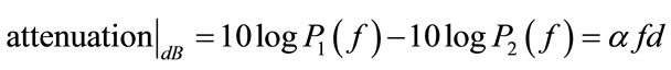
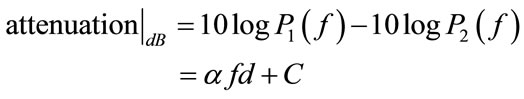
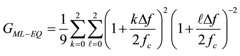
Ultrasound attenuation is the energy loss of signal after propagating through a medium. For the medium of soft tissue, Kuc assumed that its attenuation coefficient is constant over the entire sample volume and the backscattering is a Gaussian random process [1]. In such case, he presented a spatial averaging method to estimate tissue attenuation coefficient (TAC), which is estimated by the power difference of tissue echoes based on the following equation [2]:
 (1)
(1)
where  and
and  are the PSD’s of echo signals at two different ranges, d is the depth of isonified tissue, f is the signal frequency and
  is the TAC. By spatial averaging, its estimation precision is bounded by the available number of spatial samples; thus the estimation error will be large, if the sampling area is small.
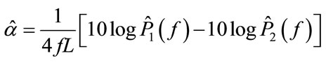
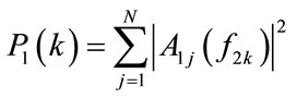
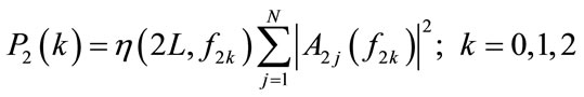
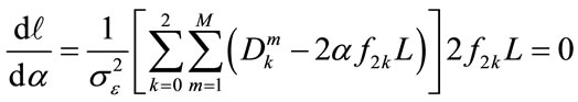
In our previews work [3], as shown in Figure 1, we proposed a method to estimate TAC of the separating tissue between two vessels using the second harmonic of microbubble, which is a single-band estimator. Assuming that the distribution of microbubbles inside the vessels are identical then we can estimate the TAC using Q independent samples of the logarithmic power as:
 (2)
(2)
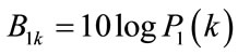
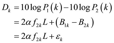
where L is the tissue length. The TAC estimate can be statistically decomposed to be:
 (3)
(3)
where  is the random error defined in [3] and rewritten in Eq.12. This estimator has a variance which can be reduced by the factor of
 . Since the Q sample are collected in time, the advantages are that the sample volume (spatial resolution) can be a small region between two vessels and the TAC can be estimated precisely
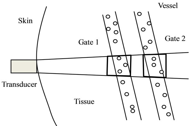
Figure 1. The schematic diagram for estimating tissue attenuation coefficient using echoes from two range gates.
using a large amount of temporally collected data; the disadvantages are that this method needs to maintain narrow band to avoid Doppler effect and it may take a long interrogation time,  (
( is the pulse repetition time), to collect Q independent samples.
Since bubbles are non-linear scatters, we may generate multiple harmonic bands of microbubbles for frequency diversity to save the interrogation time. In case K diversity frequencies are available for each transmission, then for M transmissions, there are 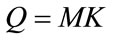 samples for estimating the TAC, which can be collected with an interrogation time of
  (
( ) only.
Theoretically, two possible strategies can be exploited to generate diversity frequencies, one is to transmit highpower pulses to generate the bubble harmonics, subharmonic and ultra-harmonics [4,5] and the other is to transmit multiple excitation frequencies as done by Newhouse et al. [6]. In general, the high-power strategy is very effective in generating bubble harmonics, however not every frequency is suitable for TAC estimation. There are two concerns in the selection of power strategy: 1) the linearity between the echo powers of bubbles at two different range gates, and 2) its effect to the life-time of bubbles.
For the linearity issue, it was found by Shi et al. [4] that powers of the first and second harmonics of bubble echo can keep a linear relation to its input acoustic pressure in double logarithmic scales; however the ultraharmonic and sub-harmonic components cannot. If this relation is nonlinear, Eq.1 will not hold any more, it will become:
 (4)
(4)
where C is an unknown bias term, since it is insonificationpower dependent. This will make TAC estimation complicated.
Another concern is the available life-time of bubbles, which limits the maximum number of pulses M. Since the ultra-harmonic and sub-harmonic components can only be generated by high insonification power, which might cause cavitation (bubble destruction) and thus reduce the life-time of bubbles. Based on these two reasons, the low-power approach given below is preferred.
Newhouse et al. [6] proposed a technique to use the nonlinear property of bubble oscillation for bubble sizing by transmitting two excitation frequencies ( and
and ) simultaneously. They derived the nonlinear response of bubble harmonic terms including the second harmonic frequencies:
  and
and , and the inter-modulation frequencies: sum frequency
  and difference frequency
 . In this approach, the bubble harmonics and inter-modulation frequencies can be generated by low power excitation, which is important to keep a linear relation between its input acoustic pressure and echo power in logarithmic scales, and keep the life-time of bubbles. The second harmonics and inter-modulation frequencies are considered to be the four diversity frequencies for developing the proposed TAC estimator with frequency diversity.
In the following sections, we analyze properties of the diversity signals and present a suitable diversity combining method for these signals to estimate TAC. To accomplish this task, a nontrivial issue about diversity frequency selection is identified. The diversity frequencies are analyzed and determined in Section 2, then we develop the diversity method and define the gains of different diversity methods in Section 3. In experimental works of Section 4, the performances of different diversity methods are verified. Finally a brief discussion and conclusion in Section 5 are presented.
2. THE DIVERSITY SIGNALS
For the low-power (multiple-excitation) approach, two important issues that affect the performance of the diversity technique are examined: 1) since multiple excitation frequencies are used, their harmonic frequencies and inter-modulated frequencies may collide (or over-lap) each other. Proper selection of the frequency spacing is required to avoid the frequency collision problem; and 2) the statistical independency of the diversity signals.
2.1. Frequency Spacing Selection
Following Newhouse’s approach, we transmit a dualfrequency signal
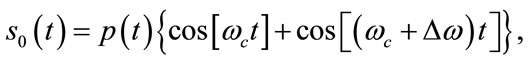
where  is the pulse envelope
  The bandwidth of
  is defined to be
 , which determines the range resolution and puts a lower bound for the frequency spacing as follows. The bubble response has four bands which are the second harmonics at
  and
and , the sum frequency at
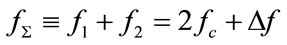
and the difference frequency at . The first three frequencies are equally spaced and
 . For convenience, these frequencies are denoted as
and called secondharmonic group also. Theoretically, the bandwidth of each frequency band is , this sets a constraint for the frequency spacing that
  must be larger than
 , i.e.,
 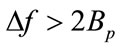 ,to avoid band overlapping.
To allow the four bubble frequencies to be useful for frequency diversity, they must be kept away from the transmitting frequencies,  and
and . A reasonable choice is to keep second-harmonic group above all transmitting frequencies, then it requires
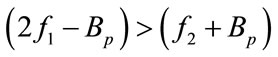 , which is equivalent to requiring that
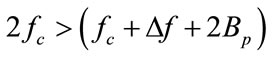 . This requirement can be simplified to be
 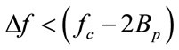 or
or . In summary, the frequency spacing must be constrained by
 , otherwise the bubble frequencies may collide the transmitting frequencies.
Based on the above constraint, it can be found that the difference frequency  is located below the transmitting bands and far away from the second harmonic group. This situation make its signal to noise ratio (SNR) be another concern in frequency spacing selection, since the bubble frequencies are located on the two ends of the transducer passband, where system gains are low. To have more bubble frequencies for diversity, a reasonable choice is to select a set of
 ,
,  and
and  such that the second harmonic group can be close to the center frequency of transducer. This choice will push the difference frequency
  close to direct current (DC), where SNR is low and thus it must be discarded. In addition, based on Eq.3, the TAC estimation error is inversely proportion to frequency; this is in favor of the second harmonic group also. Therefore, in this paper, we choose only the second harmonic group to be the diversity frequencies.
2.2. Independency of Diversity Signals
To evaluate the performance of the proposed TAC diversity estimator, the stochastic properties of the diversity signals must be known. Using the notations defined in [3] and referring to Figure 1, for the frequency  the bubble echo attenuated by a tissue (i.e. echo from vessel 2) with length L is:
 (5)
(5)
where 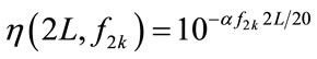 is the tissue attenuation factor at
  and
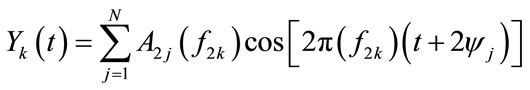
and  is the pre-attenuated bubble echo (i.e. bubble echo in vessel 1):
 (6)
(6)
where  is the scattering coefficient and
  is the time delay of the j-th microbubble.
  is a random bubble response, which depends on bubble radius
  and other physical constants.
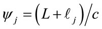 , where
  is the length between transducer and the j-th microbubble in a range-gated vessel and c is the sound speed.
Before checking the independency of the diversity signals, their correlation property is derived first. The correlation of the two pre-attenuated signals,  and
and , is:
, is:
 (7)
(7)
Since the time delay  is uniformly distributed in blood flow, its associated phase will be a uniform distribution in
 . In such case,
 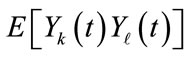 would be zero for
 , which results in that each two frequency bands are uncorrelated. When the number of bubble N is large,
  will be a zero mean Gaussian random process, then we can summarize that
  and
and  are independent to each other. By the same way, we can further show that
  and
and  are independent also, since attenuation is not a random factor.
3. DIVERSITY METHOD
Based on the TAC estimator developed in [3], there are different places to do diversity combing. Corresponding to the stages of signal processing, three possible diversity combining methods can be developed. The diversity signals may be combined at 1) power, 2) difference of logarithmic power or 3) TAC of each single-band estimate. Their differences are in combining method and available diversity gain. The combining method depends primarily on the statistical properties of the three quantities above. After analyzing the joint distribution of the multiple-frequency observations, the proposed combining method will be given in 3.1.
For the first combining method, let  be power of the pre-attenuated signal
  and
and  be power of the attenuated signal
  at the frequency
 , they can be expressed explicitly as:
 (8)
(8)
 (9)
(9)
Based on the results in [4], the samples of  and
and  follow chi-square distribution with two degree of freedom. In this case, joint distribution of the ratio of
  to
to  is asymmetric and non-central. Since the joint distributions are frequency dependent, it’s difficult to develop a TAC estimator. This is why estimator for this method is not developed.
For the second combining method, there is no such difficulty as the first one due to the logarithmic transform. Taking the logarithm of the  and
and  given in Eq.8 and Eq.9, we have
 (10)
(10)
 (11)
(11)
They are the pre-attenuated logarithmic-power of bubble echoes from vessel 1 and 2 and they have a same probability density function (pdf). Both  and
and  have non-central and asymmetric distributions. For convenience, we define the difference of the logarithmicpowers to be:
 (12)
(12)
where 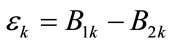 is the pre-attenuated logarithmicpower difference of the bubble signals from two vessels. Follow Kuc’s approach, when
  and
and  have the same pdf, then
  can be approximated to be a zero mean Gaussian random variable with a same variance
  for all k. Since Dk’s are independent Gaussian, their joint distribution is:
 (13)
(13)
Using this distribution, it is possible to find a maximum likelihood estimator (MLE) for the TAC, which is to be developed in Subsection 3.1.
For the third combining method, since it is done after the TAC of each band is found, a simple average is sufficient to provide a reasonable diversity estimate, which is named equal-diversity estimator. Its performance will be analyzed at 3.2.
3.1. The ML Combiner
To estimate TAC precisely we need enough statistic samples. Since the bubble scattering process is ergodic in time, we can collect M independent echoes for each diversity signal. For convenience, we rewrite the difference of the logarithmic-power for each diversity signal to be:
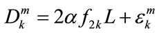 (14)
(14)
Based on the joint pdf of Eq.13, a likelihood function of the  can be found to be:
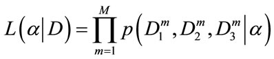 (15)
(15)
Applying Eq.13 to Eq.15, the log like-lihood function of  can be found to be:
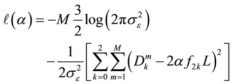 (16)
(16)
Then the MLE of  can be found by solving:
 (17)
(17)
The resultant ML estimate of TAC is:
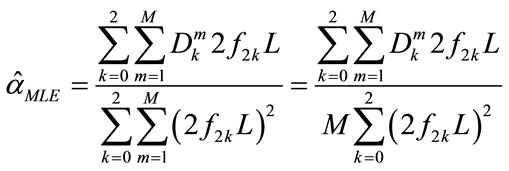 (18)
(18)
which is unbiased with the following variance:
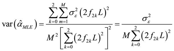 (19)
(19)
This estimator is asymptotically consistent, since
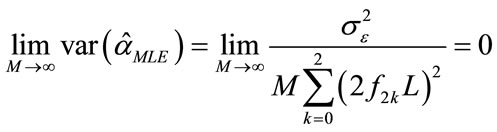 (20)
(20)
To summarize, the properties of this estimator are:
1) The multi-band TAC estimator Equation (18) will be unbiased, if the microbubbles inside vessel1 and vessel 2 have identical distribution such that  can be approximated to have a Gaussian pdf. If this condition is not hold, not only the estimation value of TAC becomes bias but also the estimation variance Eq.19 will be increased by an amount of
 .
.
2) This TAC estimator is asymptotically consistent, the estimation variance can be reduced by increasing the number of pulses M and/or the number of diversity frequencies. It means that we can use a small number of pulses to get a desired precision using frequency diversity, thus the estimation time can be saved.
3.2. Diversity Gain
In last section we have already developed a multi-band ML estimator, this section we will discuss the differences between this multi-band MLE and other diversity methods based on their diversity gain. Since the efficiency of a TAC estimator can be represented by its estimation variance, diversity gain can be defined as the inverse ratio of the variance of a multi-band MLE to that of a single-band estimator. This section is composed of 1) diversity gain of the multi-band ML estimator and 2) comparison of the difference between the equal-diversity estimator Eq.23 and the multi-band ML estimator Eq.18.
In the previous work [3], we showed that the variance of the single-band TAC estimator Eq.2 is:
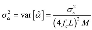 (21)
(21)
Its value is frequency dependent. Since the distribution of Eq.3 is Gaussian, the single-band TAC estimator is a ML estimator also. For quantifying the performance of the multi-band ML estimator, its diversity gain is defined to be the inverse of the ratio of its variance Eq.19 to Eq.21 as:
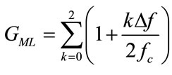 (22)
(22)
This result shows that larger frequency spacing ( ) will yield larger diversity gain.
For the third combining method in Section 3, it is the equal-diversity estimator:
 (23)
(23)
where  is the single-band TAC estimator Eq.3 for frequency =
 . Comparing to the multi-band MLE of Eq.18, the equal-diversity estimator is easy to implement. This estimator can be rewritten as:
 (24)
(24)
Its variance is equivalent to the average variance of the single-band estimator given in Eq.3. The diversity gain of the equal-diversity estimator can be found to be:
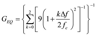 (25)
(25)
To compare these two diversity strategies, we can calculate the ratio their diversity gains given in Eq.22 and Eq.25:
 (26)
(26)
The value of  is very close to 1.0, if
  is sufficiently small or the number of diversity frequencies is large. Such case happens when bandwidth of the diversity signal is small, then performance of the ML combiner approaches that of the equaldiversity combiner.
4. EXPERIMENT
A simple in vitro experimental system is built to verify the estimation efficiency that can be improved by frequency diversity. In this experiment, we like to 1) check the correlation of diversity signals and different pulse M 2) check the consistency and the convergence rate with and without diversity 3) compare the diversity gain of the multi-band MLE to the single-band estimator and 4) compare efficiency of the multi-band MLE to the equaldiversity combiner.
4.1. Experimental Setup
The block diagram of the experimental system is presented in Figure 2. Figure 3 present the phantom of Figure 2, which is made by jelly T (Juliana, Taiwan) because this material has low acoustic attenuation. The phantom has two flows to produce two gated signals as given in Figure 1. The diameter of the flows is 5 mm. Since the phantom is soft and may be dissolved by flow, to maintain the structure the thickness of the tubes is set to be 1 mm. To avoid shadowing effect of flow 1, these two flows are positioned at different elevations within
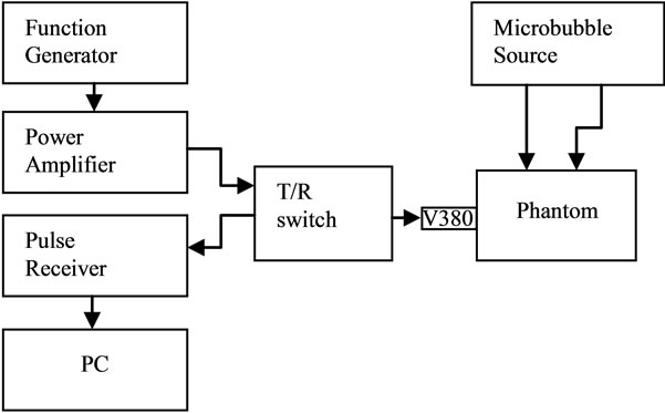
Figure 2. The block diagram of experimental system.
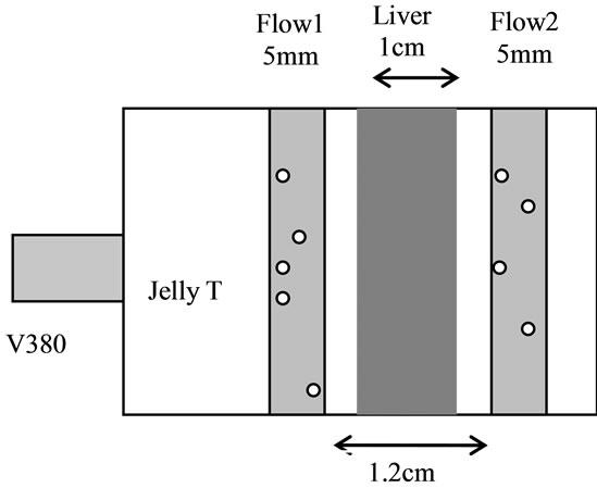
Figure 3. The phantom is made by Jelly T, which has low acoustic impedance. A fresh pork liver used for estimating TAC. The contrast agent used is Sonovue. An intravenous drip is used to simulate microbubbles in blood flow.
the beam width. Between these two flows, a fresh pork liver with a thickness of 1 cm is inserted to introduce the desired attenuation for flow 2. Pork liver is selected because it has almost constant TAC over entire region; it helps in checking the consistency and convergence rate of estimators. Before experiment, the pork liver is degassed by a vacuum machine for two hours to avoid free gas interference. The contrast agent (microbubble) used is Sonovue (BRACCO, Milan Italy). Its concentration is 10 ml in 4.5 liters of dextrose solution. An intravenous drip is used to simulate microbubbles in blood flow. A single transducer is used for both transmitting and receiving. The transducer is slicked on the phantom where the distance between flow1 and transducer is 5 cm.
The transmitter uses an arbitrary function generator (TGA1242, Thurlby Thandar Instruments Ltd., Huntingdon, England) to generate signals. Then a power amplifier (75A250 Amplifier Research, USA) is used to control the signal before applying to the T/R switch and piston probe, which is a non-focused transducer (V380, 3.5 MHz, 2.5 cm, Panametrics Waltham, MA, USA). and amplified by a low-noise amplifier (5072 PR Panametrics Waltham, MA, USA) before A/D conversion (ADLink, PCI-9812, 20MHz, 16-bit, Taiwan) The digitalized signals were stored in the PC for further processing.
In the experiment, a dual-frequency signal with center frequencies 1.5, and 2 MHz are transmitted to measure the echo signals of two bubble flows. These frequencies are selected to maintain the transducer gain at second harmonic bands. The diversity frequencies are 3, 3.5 and 4 MHz. In the experiment, the flow width is 5 mm and flow separation is 12 mm. The bandwidth of transmission signal is selected to be 100 KHz, which has a range resolution of 8 mm. Two conditions are achieved by this choice. Firstly, it makes the flows be resolvable. Secondly, it makes the flows act like point sources in range. This ensures that the bubble harmonics can be extracted in the spectrum of the range-gated flow echo. The transmission power is set at a level to make the bubbles generate second harmonics with SNR around 10 dB. The acoustic pressure is around 455 Kpa, which is measured by a hydrophone (NP-1000 PVDF needle hydrophone, TNU001A, NTR systems Inc., Seattle, WA) connected to a 30-dB preamplifier (NTR Systems Inc.).
The PRF is set at 1 KHz to ensure the independency of each sample. The flow speed is about 2.45 m/s, which is slightly faster than blood flow. A fixed flow speed helps in comparing the estimation efficiencies of different estimators. For each frequency, the measurement is repeated for 2000 times to get 2000 A-lines. Each A-line sample use a rectangular window to select the echo from flow1 and flow 2. Each windowed signal is processed according to Eq.10 and Eq.11 by FFT. The peak values of frequencies in the second-harmonic group are read to estimate TAC using Eq.18.
4.2. Experimental Results
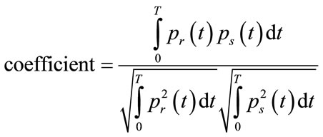
Before we check the performances of diversity estimator and single-band estimator, firstly we show the correlation property in both time domain (pulse to pulse) and frequency domain (diversity frequencies using Equation (7)) for the second harmonic group. Figure 4 present the signals of second harmonic group for successive five echoes. These signals are extracted by a Gaussian shape filter with center frequency being 3.5 MHz and bandwidth being 1.2 MHz (i.e.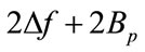 ). The waveforms look different to each other. To check the correlation quantitatively we introduce a correlation coefficient of two pulses as:
 (27)
(27)
where  and
and  are the r-th and s-th pulse echoes. The correlation coefficient of pulse 1 to others are are –0.2520, 0.4374, –0.3895 and –0.1197. These results can be considered as low correlation.
To check the property of the diversity signals, we calculate the cross correlation function of Eq.7 using 2000 pulse echoes. The diversity signals are extracted by three Gaussian filters with center frequencies: f21 = 3 MHz, f22 = 3.5 MHz and f23 =4 MHz. The correlation function are estimated by sample mean method:
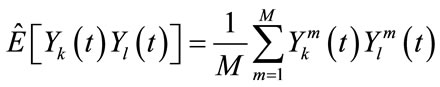 (28)
(28)
where  and
and  are the m-th samples of
  and
and . Figure 5 present the correlation function of
 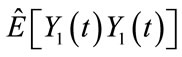 and
and . In this figure, the
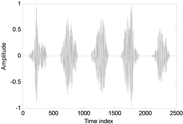
Figure 4. Pulse echo signals of second harmonic group of nearby five echoes. In this case, the correlation coefficient of pulse1 to other pulse are –0.2520, 0.4374, –0.3895 and –0.1197.
self-correlation function is much greater than cross-correlation function. The oscillation of cross-correlation is due to difference frequency components in Eq.7. Figure 6 presents the correlation functions of the three frequency components. In this figure, it demonstrates that the intensity correlation can be reduced by increasing frequency spacing (i.e., difference frequency).
Before we show that the TAC estimator Eq.18 can converge efficiently, firstly we show the converge property using the single-band estimator Eq.3. The experimental data were partitioned to have different number of pulses M for estimating the TAC. Figure 7(a) presents the estimated TAC values using the second harmonic frequency fc = 3 MHz. For M < 2000, there are multiple sub-sets of data for estimating the TAC. The different estimates are presents as scatter diagrams for M = 5, 25, 50, 100, 500, 1000, 1500 and 2000 in Figure 7(a). The estimate values are spread between –0.5 and 1.6  when M = 5, finally
  converges to 0.4890
  when M is increased to 2000. In this case, we prove that Eq.20 is attained when pulse number M is increased.
To check 2), Figure 7(b) presents the TAC estimation values of the multi-band MLE Eq.18 using data of 3, 3.5 and 4 MHz. In this figure, the estimation values converge as the number of pulses M increases. This estimator converges consistently as M increased to 2000. The converged value is 0.504 , this value is very close to the single-band estimation value. This shows that Eq.18 is also an unbiased estimator. Compare to Figure 7(a), the variation of multi-band MLE at each M is smaller than that of single-band estimator, this is because that each pulse has three samples in multi-band MLE. This shows that Eq.20 is attained.

Figure 5. Correlation function of  (upper) and
  (lower) which are calculated by 2000 samples. This figure present cross-correlation of two different diversity frequency is much smaller than correlation of the same diversity frequency.

Figure 6. Cross-correlation function of ,
,  and
and . These three figures shows that the main component of correlation function (7) is the difference frequency term. The intensity of correlation can be reduced by increasing frequency spacing.
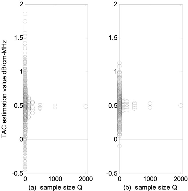
Figure 7. The distribution of estimation values of single band (3M Hz) and multiband (3, 3.5 and 4 MHz) estimators.
To check the convergence property of using singlefrequency estimator (3 MHz) and three-frequency estimator (3, 3.5 and 4 MHz), we calculate the estimation variance with M = [10, 25, 50, 100]. The variances of the three-frequency estimator are: 0.0222, 0.0084, 0.0041 and 0.0028 . The variances of the singlefrequency estimator are: 0.0958, 0.0341, 0.0189 and 0.0087
 . These results shows 1) both estimators converge according to 1/M and 2) the diversity technique works effectively in all cases, since each variance ratio at certain M are approximately 4.18. This result also shows that both time domain and frequency domain samples can be considered to be independent samples.
Table 1 can be used to check the diversity gain when using two frequencies and three frequencies for diversity combining. Since the diversity gain can be calculated by Eq.22 as the variance ratio of different estimators and their values are independent of the number of pulses M. We select M = 5 for the estimators to calculate their variances. In this case, each variance value is calculated using 400 realizations. For simplicity, we select variance ratio of the single-frequency estimator (3 MHz) and the two-frequency estimator (3 & 4 MHz) to represent the diversity gain of MLE using two frequencies. Theoretical value of this ratio is 2.8 using Eq.22 and the experimental value is 3.1 (0.188/0.059), which is slightly greater than theoretical value. This is because that the variance  is not a constant value for each frequency. Another case is diversity gain of MLE using three frequencies. The theoretical value is 4.14 using Eq.22, which is also smaller than the experimental value 4.18 (0.188/0.045). Based on these results, we can conclude that the estimation variance can be decreased by increasing frequency bands or using higher frequency for estimation.
To check 4), the variances of two diversity methods, MLE Eq.18 and equal-diversity Eq.23, are given in Table 2. All variance values are calculated using 400 realizations of data. The results show that the estimation variances of equal diversity are slightly larger (10%) than those of MLE. This is due to that the value of  is
is  in this experiment, which are small values for
 . This result confirms the relation given by Eq.26.
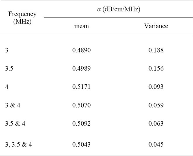
Table 1. Statistics of the estimated tac using the multiple second harmonic bands. Estimation variance is used to check efficiency of each estimator. The sample size Q is 2000 for all cases.
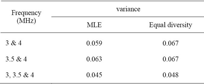
Table 2. Estimation variance of equal diversity and MLE The results show that the estimation variances of equal diversity are slightly larger (10%) than those of MLE. The Sample Size Q is 5 with 400 estimated values for All Cases.
In this experiment, since the estimation variance of equal diversity is slightly larger than MLE and the estimation variance is quite small so that we can use equal diversity to estimate TAC.
5. DISCUSSION AND CONCLUSION
In this paper, the single-frequency TAC estimator [4] is extended to be a multiple-frequency diversity estimator using bubble harmonics. First we developed a strategy to select suitable frequency bands for diversity; we also model the stochastic attenuation model for the diversity frequencies. We presented a MLE of TAC for these frequency bands and compare its efficiency to that of the linear-diversity estimator, which is the simplest diversity strategy.
In the experimental work, we use a dual-frequency signal to verify this technique. The experimental results show that the frequency diversity works well, which confirms that the assumption of independency for each frequency band is proper. By checking efficiency of the diversity technique, it is found that the variance of logarithmic-power  is frequency dependent and much smaller than what Kuc presented [1]. In the future, we like to check the physical and statistical properties of bubble echoes and present a statistical model for
 .
.
Another consideration is about the usage of the difference-frequency band, in this paper this band is discarded due to frequency collision and low SNR. If we can overcome these problems, this frequency band can still have diversity gain and a MLE include this band can be developed.
Theoretically the TAC estimator may be affected by transducer bandwidth, beam width, vessel size, distance between vessels, and bubble density mismatch. To compensate these effects is a possible further development.
Another possible further development is about the use of more than two excitation frequencies to increase number of diversity signals. In such case, a more complicated frequency-collision problem may occur in the differencefrequency band. For example, if we transmit a threefrequency signal with frequencies: ,
,  and
and , the bubble echo will consist of two difference-frequency signals as:
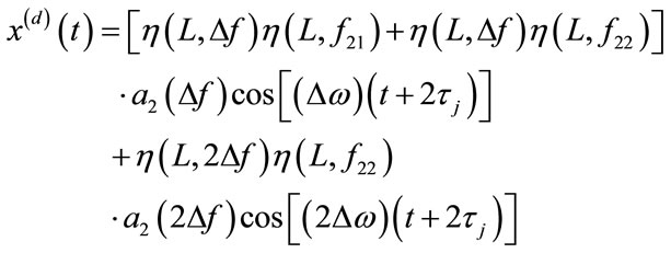 (29)
(29)
It is noted that the first component of Eq.29 consists of two different attenuation quantities, therefore it can not be used for TAC estimation; only the second component is useful.
In this paper, we have already increased the estimation efficiency of TAC estimation using multiple bubble harmonics. For completeness, this method may need estimators for other parameters, e.g., tissue length estimator, and need experimental works to demonstrate in vivo applacations [7].
![]()
![]()
REFERENCES
- Kuc, R. and Schwartz, M. (1979) Estimating the acoustic attenuation coefficient slope for liver from reflected ultrasound signals. IEEE Transactions on Sonics and Ultrasonics, SU-26, 353-362. doi:10.1109/T-SU.1979.31116
- Kuc, R. (1984) Estimating acoustic attenuation from reflected ultrasound signals: Comparison of spectral-shift and spectral-difference approaches. IEEE Transactions on Acoustics, Speech and Signal Processing, 32, 1-6. doi:10.1109/TASSP.1984.1164282
- Tsao, S.K. and Tsao, J. (2010) A consistent tissue attenuation coefficient estimator using bubble harmonic echoes. IEEE Transactions on Ultrasonics Ferroelectrics and Frequency Control, 57, 2654-2661.
- Shi, W.T. and Forsberg, F. (2000) Ultrasonic characterization of the nonlinear properties of contrast microbubbles. Ultrasound in Medicine and Biology, 26, 93-104. doi:10.1016/S0301-5629(99)00117-9
- Miller, D.L. (1978) Ultrasounic detection of resonant cavitation bubbles in a flow tube by their second-harmonic emissions, Ultrasonics, 19, 217-224.
- Newhouse, V.L. and Shankar, P.M. (1984) Bubble size measurements using the nonlinear mixing of two frequencies. Journal of Acoustical Society of America, 75, 1473-1477. doi:10.1121/1.390863
- Bridal, S.L., Beyssen, B., Fornes, P., Julia, P. and Berger, G. (2000) Multiparametric attenuation and backscatter images for characterization of carotid plaque. Ultrasonic Imaging, 22, 20-34.
NOTES
*This work was supported by the National Science Council, Taipei, Taiwan (NSC100-2221-E-002-063).