Intelligent Information Management
Vol.2 No.4(2010), Article ID:1720,9 pages DOI:10.4236/iim.2010.23033
Tracking with Estimate-Conditioned Debiased 2-D Converted Measurements
1Cobham Analytic Solutions, Huntsville, USA
2Department of Electrical and Computer Engineering, University of Alabama in Huntsville, Huntsville, USA
E-mail: john.spitzmiller@cobham.com, adhami@ece.uah.edu
Received January 16, 2010; revised February 27, 2010; accepted April 1, 2010
Keywords: Tracking, Converted Measurements, Kalman Filter, Unscented Transformation
Abstract
This paper describes a new algorithm for the 2D converted-measurement Kalman filter (CMKF) which estimates a target’s Cartesian state given polar position measurements. At each processing index, the new algorithm chooses the more accurate of (1) the sensor’s polar position measurement and (2) the CMKF’s Cartesian position prediction. The new algorithm then computes the raw converted measurement’s error bias and the corresponding debiased converted measurement’s error covariance conditioned on the chosen position estimate. The paper derives explicit expressions for the polar-measurement-conditioned bias and covariance and shows the resulting polar-measurement-conditioned CMKF’s mathematical equivalence with the 2D modified unbiased CMKF (MUCMKF). The paper also describes a method, based upon the unscented transformation, for approximating the raw converted measurement’s error bias and the debiased converted measurement’s error covariance conditioned on the CMKF’s Cartesian position prediction. Simulation results demonstrate the new CMKF’s improved tracking performance and statistical credibility as compared to those of the 2D MUCMKF.
1. Introduction
The converted-measurement Kalman filter (CMKF) is a popular solution to the nonlinear-estimation problem of tracking a target, whose 2D kinematics are described in Cartesian coordinates, given polar position measurements [1-3]. The 2D CMKF algorithm converts the polar position measurement to Cartesian coordinates using the familiar nonlinear mapping between the two coordinate systems, yielding a measurement model that is a linear function of the target’s Cartesian state. The CMKF then performs target tracking entirely in Cartesian coordinates using the classical Kalman-filtering algorithm.
As shown in [1], the nonlinear transformation of an unbiased polar measurement to a raw Cartesian converted measurement creates a bias in the raw converted measurement’s error. Debiasing the raw converted measurement with this bias produces an unbiased converted measurement for the classical Kalman-filter tracking algorithm. After the raw converted measurement is debiased, the CMKF algorithm requires only the accurate determination of the debiased converted measurement’s error covariance to employ the classical Kalman-filter tracking algorithm to maximum effect.
Lerro and Bar-Shalom’s original work in this area [1] derived explicit expressions for the raw converted measurement’s true error bias and the debiased converted measurement’s true error covariance. Debiasing the raw converted measurement with the raw converted measurement’s true bias and employing the debiased converted measurement’s true error covariance in the classical Kalman-filter tracking algorithm comprise the ideal debiased 2D CMKF algorithm. However, Lerro and BarShalom showed the true bias and covariance to be functions of the target’s true position coordinates which are clearly unavailable in practice. In response to this obvious problem, Lerro and Bar-Shalom conditioned the mean of the raw converted measurement’s true error bias and the mean of the debiased converted measurement’s true error covariance on the readily available polar measurement to obtain practical bias and covariance approximations.
The unbiased CMKF (UCMKF) subsequently developed by L. B. Mo, X. Q. Song, et al. [2] utilized a practical measurement conversion that produced an unbiased converted measurement by multiplying the raw converted measurement by a vector of bias-elimination factors. However, L. B. Mo, X. Q. Song, et al. showed the unbiased converted measurement’s true error covariance to be a function of the target’s true position. The UCMKF’s corresponding practical approximation to the unbiased converted measurement’s true error covariance resulted from conditioning the covariance of the unbiased converted measurement (rather than the unbiased converted measurement’s error) on the polar measurement.
Duan, Han, and Li [3] later showed the approach of [2] to have a mathematical incompatibility between the derivations of the UCMKF’s unbiased converted measurement and approximate converted-measurement error covariance. Duan, Han, and Li’s corrected algorithm, now known as the modified unbiased CMKF (MUCMKF), debiased the UCMKF’s already unbiased converted measurement with the polar-measurement-conditioned unbiased converted measurement’s error bias. Additionally, Duan, Han, and Li derived the corresponding converted-measurement-error covariance conditioned strictly on the polar measurement to complete the MUCMKF’s specifications.
This paper describes an innovative yet practical CMKF algorithm which more accurately emulates Lerro and Bar-Shalom’s ideal debiased 2D CMKF. Specifically, the new CMKF algorithm uses a three-stage process to compute the essential converted-measurement-error statistics conditioned on the more accurate of the two practically available target-position estimates rather than exclusively on the polar position measurement. First, at each processing index, the new CMKF algorithm determines the more accurate of (1) the sensor’s polar position measurement and (2) the CMKF’s Cartesian position prediction. Second, the new CMKF algorithm calculates the raw converted measurement’s error bias conditioned on the chosen target-position estimate; the new CMKF algorithm then debiases the raw converted measurement with this calculated bias. Third, the new CMKF algorithm calculates the debiased converted measurement’s error covariance conditioned on the chosen target-position estimate. The paper shows the CMKF algorithm which results from conditioning the raw converted measurement’s error bias and the corresponding debiased converted measurement’s error covariance exclusively on the polar measurement to be mathematically equivalent to the 2D MUCMKF. More importantly, the paper proposes a novel method, based on the unscented transformation (UT) [4], for closely approximating the raw converted measurement’s error bias and the corresponding debiased converted measurement’s error covariance conditioned on the CMKF’s Cartesian position prediction since this target-position estimate is often more accurate than the sensor’s polar position measurement [1].
Section 2 reviews the technical background germane to polar-to-Cartesian measurement conversion and its application to the CMKF. Section 3 provides a detailed mathematical description of the new CMKF algorithm. Section 4 presents simulation results which demonstrate the new CMKF algorithm’s improved tracking performance and statistical credibility over those of the 2D MUCMKF. Section 4 also compares the computational requirements of the new CMKF algorithm with those of the 2D MUCMKF algorithm. Section 5 summarizes the paper’s significant contributions and the new CMKF algorithm’s advantages and disadvantages.
2. Technical Background
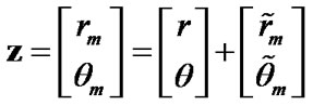
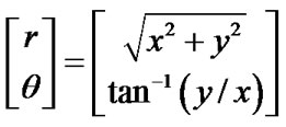
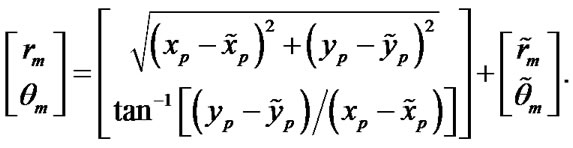
A sensor measures a target’s position and produces the polar position measurement
 (1)
(1)
In (1),  is the target’s true position in polar coordinates (range and bearing), and
  is a white, zero-mean, Gaussian measurement noise with covariance
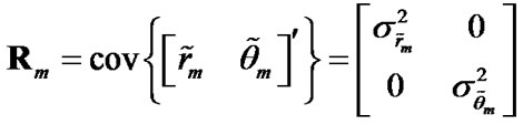 (2)
(2)
Since the target’s true Cartesian position is
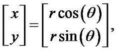 (3)
(3)
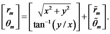
the error  of the raw converted measurement
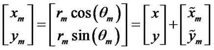 (4)
(4)
is
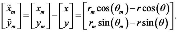 (5)
(5)
Lerro and Bar-Shalom [1] derived the raw converted measurement’s true error bias
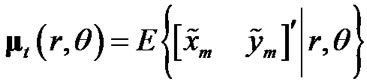 (6)
(6)
with which (4) can be debiased to produce an unbiased converted measurement. They also derived the corresponding debiased converted measurement’s true error covariance
 (7)
(7)
which is necessary for the classical Kalman-filter algorithm. However, since (6) and (7) depend upon the target’s true range and bearing, realizable CMKFs cannot use these expressions. The next section presents a new approach to practically approximating (6) and (7).
3. The New CMKF Algorithm
This section develops a new 2D CMKF algorithm in three parts on the assumption that better CMKF performance results from conditioning the raw converted measurement’s error bias and the debiased converted measurement’s error covariance on the most accurate available target-position estimate. The first part derives explicit expressions for the raw converted measurement’s error bias and the debiased converted measurement’s error covariance, when those quantities are conditioned on the polar measurement. This part also shows the corresponding polar-measurement-conditioned CMKF to be mathematically equivalent to the 2D MUCMKF. The second part presents a technique, based on applications of the UT, for closely approximating the raw converted measurement’s error bias and the debiased converted measurement’s error covariance conditioned on the CMKF’s Cartesian position prediction. The third part describes a test which, for each processing index, chooses between the sensor’s polar position measurement and the CMKF’s Cartesian position prediction for the target-position estimate on which the raw converted measurement’s error bias and the debiased converted measurement’s error covariance should be conditioned.
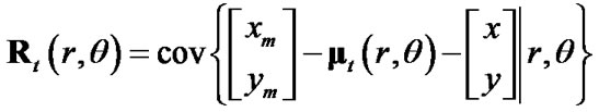
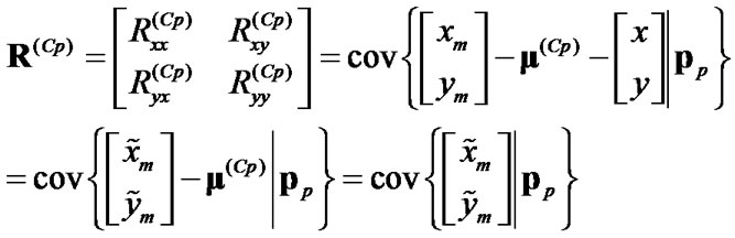
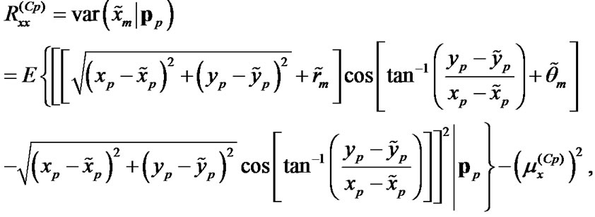
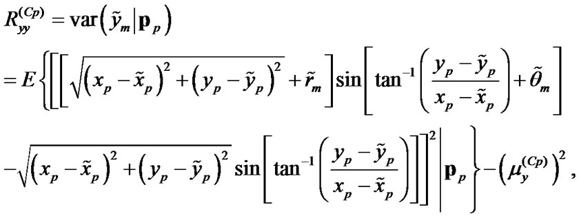
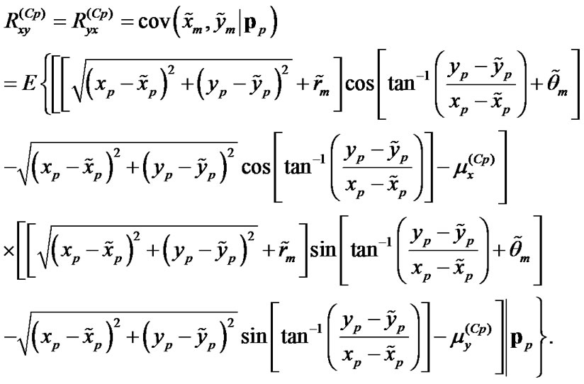
3.1. Converted-Measurement-Error Statistics Conditioned on the Sensor’s Polar Position Measurement
The polar-measurement-conditioned bias of the raw converted measurement’s error is
 (8)
(8)
with elements
 (9)
(9)
and
 (10)
(10)
Using basic trigonometric identities and (5) of [1], we simplify (9) and (10) to
 (11)
(11)
and
 (12)
(12)
respectively. The corresponding polar-measurementconditioned covariance of the debiased converted measurement’s error is
 (13)
(13)
with elements
 (14)
(14)
 (15)
(15)
and
 (16)
(16)
Using basic trigonometric identities and (5) of [1], we simplify (14)–(16) to
 (17)
(17)
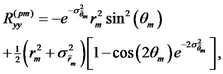 (18)
(18)
and
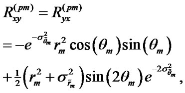 (19)
(19)
respectively.
From (12) of [2],
 (20)
(20)
and
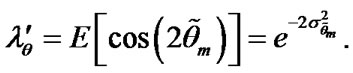 (21)
(21)
Substituting (20) and (21) into (17)-(19) produces precisely the elements of Rp, the 2D MUCMKF’s converted-measurement-error covariance [3]. Furthermore, the 2D MUCMKF’s final converted-measurement elements are specified as [3]
 (22)
(22)
and
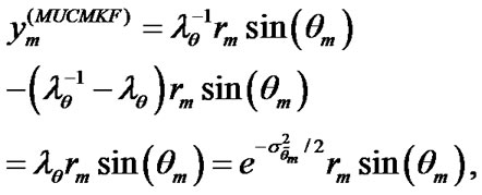 (23)
(23)
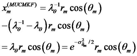
and the polar-measurement-conditioned debiased converted-measurement elements of the new CMKF algorithm are
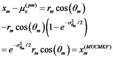 (24)
(24)
and
 (25)
(25)
Given a particular target-kinematics model and a particular filter-initialization method, a CMKF algorithm’s full description requires only (1) the final form of the converted measurement (whether raw, debiased, or unbiased) and (2) the employed error covariance of the converted measurement’s final form. Thus, the CMKF algorithm which results from conditioning the raw converted measurement’s error bias and the debiased converted measurement’s error covariance exclusively on the polar measurement is mathematically equivalent to the 2D MUCMKF since both algorithms use exactly the same final converted-measurement form and exactly the same converted-measurement error covariance.
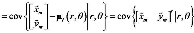
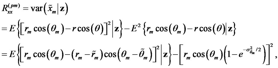
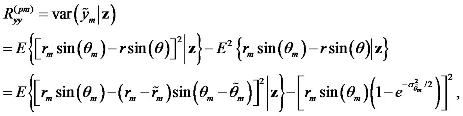
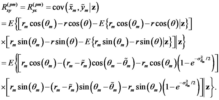
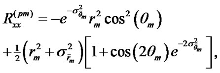
3.2. Converted-Measurement-Error Statistics Conditioned on the CMKF’s Cartesian Position Prediction
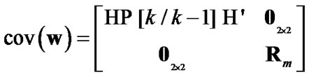
This section describes a technique for conditioning the raw converted measurement’s error bias and the debiased converted measurement’s error covariance on the CMKF’s Cartesian position prediction. To obtain the desired bias and covariance expressions, we first assume the CMKF’s Cartesian position prediction can be modeled as
 (26)
(26)
where  is a zero-mean error with covariance
 (27)
(27)
We use the covariance of the position elements of the CMKF’s Cartesian state prediction as a practically available approximation to (27). Mathematically, at processing index ,
,
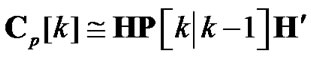 (28)
(28)
where
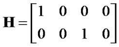 (29)
(29)
is the 2D CMKF’s measurement matrix [1] and  is the CMKF’s predicted state-estimate-error covariance.
The target’s true polar position is related to its true Cartesian position with
 (30)
(30)
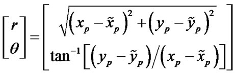
Substituting (30) into (1) yields
 (31)
(31)
Solving (26) for [x y]’ and substituting the result into (30) and (31) yield
 (32)
(32)
and
 (33)
(33)
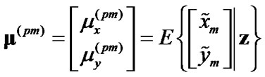
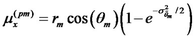
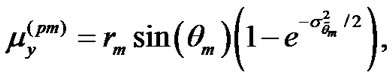
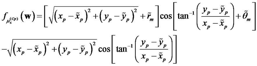
Using the elements of (32) and (33), the raw converted measurement’s error bias, when conditioned on the CMKF’s Cartesian position prediction, is
 (34)
(34)
with elements
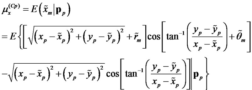 (35)
(35)
and
 (36)
(36)
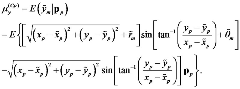
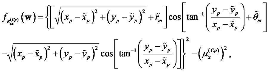
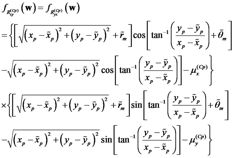
The corresponding debiased converted measurement’s error covariance, when conditioned on the CMKF’s Cartesian position prediction, is
 (37)
(37)
with elements
 (38)
(38)
 (39)
(39)
and
 (40)
(40)
Since the Cartesian position prediction’s error has an unknown joint density and a generally non-diagonal covariance, we cannot obtain simple, closed-form solutions for (35), (36), and (38)-(40). Thus, some non-analytical means of computing or at least approximating (35), (36), and (38)–(40) is required. Since these expressions all represent expectations of nonlinear transformations of the random vector
 (41)
(41)
we propose applying the UT to the problem of approximating the output-distribution means of the nonlinear functions within the expectation operators of (35), (36) and (38)-(40) given the mean and covariance of w.
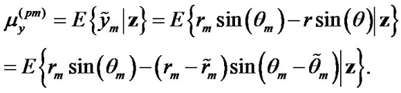
Whereas the polar measurement’s noise  is known to be jointly Gaussian, the Cartesian position prediction’s error
  has a joint density that is both unknown and likely unknowable. We therefore assume the joint density of (41) to be approximately Gaussian with mean
  and covariance
 (42)
(42)
since, relative to the true target position, the polar measurement’s noise is uncorrelated with the Cartesian prediction’s error. Since , the vector at the input of the nonlinear transformations within the expectation operators of (35),(36) and (38)-(40), has dimension four, we generate the nine sigma points and the nine weights given by (3) of [4] with a choice of
  to satisfy the given heuristic. Using the generated sigma points and weights, we then calculate with (4) of [4] the UT-approximated output-distribution means of the nonlinear functions
 (43)
(43)
and
 (44)
(44)
as approximations to  and
and , respectively.
Using the same nine sigma points generated to approximate  and
and , we calculate the UT-approximated output-distribution means of the nonlinear functions.
 (45)
(45)
 (46)
(46)
and
 (47)
(47)
as approximations to ,
,  , and
, and respectively. Note that the UT-calculated output-distribution mean values of (43) and (44) are respectively substituted for
  and
and  in (45)-(47).
3.3. Choosing the Target-Position Estimate for Bias and Covariance Conditioning
This section describes a decision metric for choosing between the sensor’s polar position measurement and the CMKF’s Cartesian position prediction for the targetposition estimate on which to condition the raw converted measurement’s error bias and the debiased converted measurement’s error covariance. Lerro and Bar-Shalom’s test (Equation (35) of [1]) represents a simple and practical method for determining the less uncertain of these two target-position estimates by comparing the sizes, as measured by the matrix determinant, of the error covariances in Cartesian coordinates. We propose a test based on a conceptually identical approach. Specifically, if the determinant of  equals or exceeds the determinant of
 , the test judges the sensor’s polar measurement as the less uncertain target-position estimate, and the new technique computes the raw converted measurement’s error bias and the debiased converted measurement’s error covariance conditioned on the sensor’s polar measurement. Otherwise, the test judges the CMKF’s Cartesian position prediction as the less uncertain target-position estimate, and the new technique (approximately) computes the raw converted measurement’s error bias and the debiased converted measurement’s error covariance conditioned on the CMKF’s Cartesian position prediction. Mathematically, the test chooses the target-position estimate used for bias and covariance conditioning according to
 (48)
(48)
4. Simulation Results
To test the performance of the new CMKF against the 2D MUCMKF, we replicate the two test cases used by [3] with 10000 Monte-Carlo runs rather than 500. Specifically, for both cases, the sensor takes 200 range and bearing measurements with a constant measurement interval of 1 s. The sensor’s range-error standard deviation is 100 m, and the bearing-error standard deviation is 2.5°. Two independent draws from a Gaussian distribution with mean 10 km and standard deviation 100 m determine the target’s initial x and y position components. Additionally, two independent draws from a Gaussian distribution with mean 20 m/s and standard deviation 10 m/s determine the target’s initial x and y velocity components. The target’s two acceleration-disturbance components are independent, white, zero-mean, Gaussian noises with standard deviation 0.01 m/s2. Case 1 uses the nearly-constant-velocity target-kinematics model (Equation (2297) of [5]) for both Cartesian dimensions. Case 2 uses the 2D nearlycoordinated-turn target-kinematics model of [6] with a known turn rate of 0.1 rad/s in the x-y plane.
Figure 1 shows overlays of the RMS position-tracking errors for the target of Case 1. Clearly the new CMKF provides superior tracking performance (as indicated by

Figure 1. RMS position-tracking errors (Case 1).
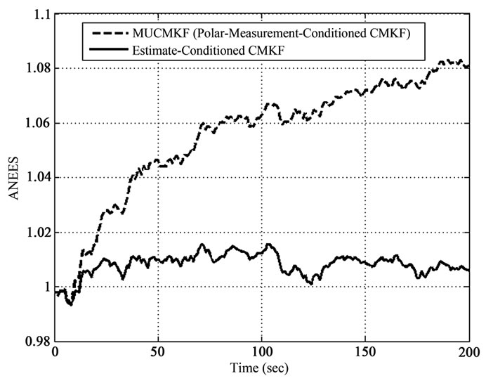
Figure 2. ANEES (Case 1).
its lower RMS position-tracking error) when compared to the 2D MUCMKF for the first considered test case.
Figure 2 shows overlays of the average normalized estimation error squared (ANEES) curves for the target of Case 1. Clearly the new CMKF provides superior credibility (as indicated by the nearer proximity of its ANEES to one) when compared to the 2D MUCMKF for this test case.
Figure 3 shows overlays of the RMS position-tracking error for the target of Case 2. Again the new CMKF provides superior tracking performance when compared to the 2D MUCMKF for the second considered test case.
Figure 4 shows overlays of the ANEES curves for the target of Case 2. Again the new CMKF provides superior credibility when compared to the 2D MUCMKF for this test case.
The 2D MUCMKF algorithm required an average time of 0.19944 ms to execute a single iteration using MATLAB version 7.4 on an Intel® Core™ 2 Duo CPU T7300 running at 1.99 GHz with 2 GB of RAM. Using
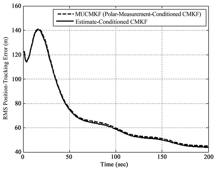
Figure 3.RMS position-tracking errors (Case 2).
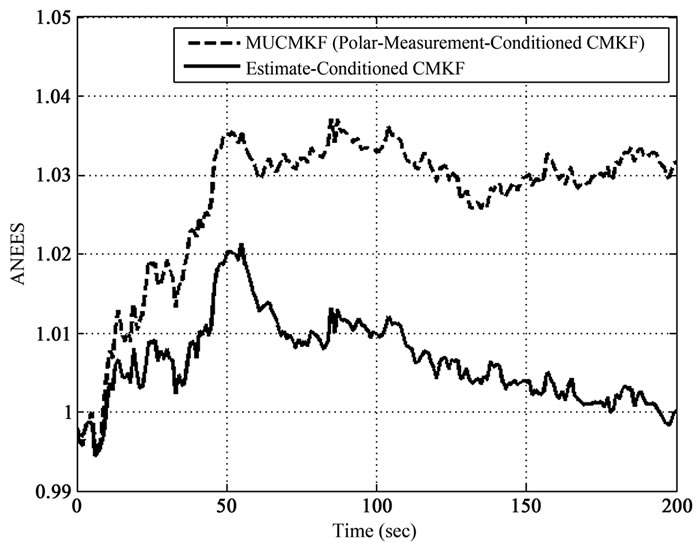
Figure 4. ANEES (Case 2).
the same hardware and software, the new CMKF algorithm required an average time of 0.22763 ms to execute a single iteration when the raw converted measurement’s error bias and the debiased converted measurement’s error covariance are conditioned on the CMKF’s Cartesian position prediction. Thus, the performance improvements shown in Figures 1-4 come at the cost of increased computational time required to compute the UT‑approximated output-distribution means.
5. Conclusions
The work documented in this paper offers four significant contributions to the field of CMKF tracking. First, the paper derives explicit expressions for the raw converted measurement’s error bias and the debiased converted measurement’s error covariance when these quantities are conditioned on the polar measurement. Second, the paper shows the application of the polar-measurement-conditioned bias and covariance expressions results in a CMKF mathematically equivalent to the 2D MUCMKF. Third, the paper describes a novel application of the UT to approximately solve the problem of conditioning the raw converted measurement’s error bias and the debiased converted measurement’s error covariance on the CMKF’s Cartesian position prediction. Fourth, the paper adapts a previously published decision metric to automatically choose the more accurate target-position estimate—either the sensor’s polar position measurement or the CMKF’s Cartesian position prediction—at each processing index, thus allowing the integration of the two conditioning techniques into a single algorithm.
The new CMKF algorithm described in this paper yields noticeably better RMS tracking performance and statistical credibility when compared with the 2D MUC-MKF or, equivalently, a 2D CMKF which conditions the raw converted measurement’s error bias and the debiased converted measurement’s error covariance strictly on the polar measurement. However, the new algorithm’s improved performance comes at the cost of additional computations required for several UT calculations since the CMKF’s Cartesian position prediction is usually more accurate than the sensor’s polar position measurement.
6. References
[1] D. Lerro and Y. Bar-Shalom, “Tracking with Debased Consistent Converted Measurements Versus EKF,” IEEE Transactions on Aerospace and Electronic Systems, Vol. 29, No. 3, 1993, pp. 1015-1022.
[2] L. B. Mo, X. Q. Song, Y. Y. Zhou, Z. K. Sun and Y. Bar-Shalom, “Unbiased Converted Measurements for Tracking,” IEEE Transactions on Aerospace and Electronic Systems, Vol. 34, No. 3, 1998, pp. 1023-1027.
[3] Z. Duan, C. Han and X. R. Li, “Comments on Unbiased Converted Measurements for Tracking,” IEEE Transactions on Aerospace and Electronic Systems, Vol. 40, No. 4, 2004, pp. 1374-1377.
[4] S. Julier, J. Uhlmann and H. F. Durrant-Whyte, “A New Method for the Nonlinear Transformation of Means and Covariances in Filters and Estimators,” IEEE Transactions on Automatic Control, Vol. 45, No. 3, 2000, pp. 477-482.
[5] Y. Bar-Shalom and T. Fortmann, “Tracking and Data Association,” Academic Press, New York, 1988.
[6] Y. Bar-Shalom and X. R. Li, “Estimation and Tracking: Principles, Techniques, and Software,” Artech House, Norwood, 1993.