iBusiness
Vol.2 No.1(2010), Article ID:1441,10 pages DOI:10.4236/ib.2010.21006
Evolution and Forecasting of Business-Centric Technoeconomics: A Time-Series Pursuit via Digital Ecology
![]()
Department of Computer & Electrical Engineering and Computer Science, Florida Atlantic University, Fort Lauderdale, USA.
Email: neelakan@fau.edu
Telecommunication Services
Received August 18th, 2009; revised October 3rd, 2009; accepted November 19th, 2009.
Keywords: Digital Ecology, Business-Centric Economics, Evolution and Forecasting, ARIMA Modeling,
ABSTRACT
Time-evolution and hence, forecasting the growth profiles of business-centric technoeconomics are ascertained. As an example, the vast telecommunication (telco)-specific business is considered as a complex enterprise depicting a cyberspace of digital ecology (DE) with a backbone of network that supports a host of information sources and destinations facilitating a variety of triple (voice, data and video) services. To specify the temporal trend of evolution of telco economics in a series format, the approach pursued here (and differs from traditional series analyses) takes into account only a selective (and justifiable) set of autoregressive integrated moving average (ARIMA) parameters consistent with the test data. However, this simplified approach yields sufficiently accurate time-series (depicting the business growth) extendable to forecasting regimes. The efficacy of the proposed method is determined via goodness-fit evaluations both in timeand frequency-domains. The data adopted in the computations conform to typical telco service industry.
1. Introduction
In modern business world, the plethora of telecommunication (telco) networks and the associated information technology (IT) is comprised of a technological infrastructure supporting streams of voice, data and video (entertainment) data flow plus an economic base that earns revenues as well as incurs capital and operational expenses (CAPEX and OPEX). In this technoeconomic context, the entirety of telco service industry constitutes a complex digital ecology (DE) populated by a set of “digital species” denoting various (tele)-communication entities (information, technology, service options etc.) along with the entirety of computing systems (softand hardware), constituents of entertainment media and items of economics. DE is a neoteric perception [1], which can be attributed to the complex system of telecommunications [2].
Within the broad scope of DE, addressed exclusively in this paper are heuristics of business-centric digital ecosystems (such as telco service industry) in ascertaining the temporal trend and seasonal/non-seasonal movements of the underlying technoeconomic parameters (expressed in terms of a time-series representation of the associated data). The approach pursued thereof differs from traditional analyses by considering only a selective set of global moving-average (such as autoregressive integrated moving average or ARIMA) parameters compatible for the test data. The reasons for selective parameter-set usage are justifiably explained.
In spite of the simplified approach (via selective parameter usage), the method indicated yields sufficiently accurate time-series depiction of business growth/evolution compatible for forecasting efforts. The efficacy of the proposed technique is determined via goodness-fit evaluations both in timeand frequency-domains. The data adopted in the computations conform to typical telecommunication (telco) service industry.
2. Technoeconomic Growth Profile
In the context of modern telco service business, modeling the associated growth scenario (viewed in terms of service expansion, revenue growth, customer population etc.) will lead to predicting the survival of the business in the cyberspace of service provisioning implicated by interacting aspects of quality-of-service (QoS) expectations, variety in services (of voice, data and video), competitive deregulated market, government regulations, customer churning, revenue/return-on-investment (RoI) etc..
Given a set of data on technoeconomic evolution, which is invariably nonlinear [3], it is governed by various endogenous and/or exogenous variables; and, a regression analysis of it can be normally performed in order to get a trend curve, which is projected to forecast an estimate of possible values of the dependent variable at any specified value of the dependent variable extrapolated beyond the range over which the regression is performed. This is called trend projection (forward) procedure. Further, forecasting is exercised via exponential smoothing of the trend projection, wherein greater weights to recent observations are prescribed in the timeseries.
Considering time-series representation of short-term growth of technoeconomics, often cyclical and/or seasonal variations (specified as what are known as seasonal indices) are seen in the trend projection. In the time-series analysis of long-term business planning issues and decision suite, such seasonal movements and variations should be explicitly included in realistic trend projections toward forecasting (because, the growth of underlying economic features is supposedly centered on such movements and trend details on such movements imply a moving average (MA) of seasonal variations). The associated seasonal indices are decided by annihilation and augmentation of details (technoeconomic information) applied on the growth function dynamics (mostly in random manner); and as such, the growth aspect of the system would exhibit a jagged variation (largely in the initial phase) caused by the (random) interactions of endogenous and/or exogenous entities) [3].
The seasonal index indicated above can be defined, for example, in terms of raw data of pertinent economic information across specified periods, (such as quarters of a year). Normally the pattern of time-series is assumed to be stable over the “season” of interest and the seasonal variations presumably follow the baseline trend. Hence, the series of successive moving averages roughly denote the trend as well as cyclic/seasonal elements. Typically, the time-series of economic variation conceived in terms of original/raw observations periodically (say, quarterly) are expressed as MA figures and data-shift components (namely, cyclical, seasonal and irregular (random) entities) [4].
Forecasting time-series typically follows the classical methodology known as X-12 procedure proposed by the US Bureau of Census [5]. It implements the strategy of segregating descriptive components into trend and cyclic movements and leads to evaluating the constants and seasonal indices of time-series data. The underlying procedure eliminates large (as well as small) outliers of the data. It also smoothens out speckles of non-informative fluctuations. That is, in estimating the parameters via X-12 procedure, relevant seasonal adjustment implies a signal-extraction technique of seasonal movements manifesting as a noise-like feature. Therefore non-informative artifacts have to be suppressed in order to reveal the signal part of interest more explicitly. A practical method that includes such signal extraction procedure is due to Box and Jenkins [6,7], which can be implemented basically by the following steps: 1) Exercising an identification procedure so as to determine whether the time-series can be specified by a combination of MA and autocorrelation terms; 2) using this combination performing an estimation of parameters of a tentative model; and 3) applying a diagnostic test to examine the adequacy of matching between fitted models vis-à-vis raw data.
In general, the technoeconomic growth trend plus the seasonal and non-seasonal variations can be modeled either in an analytical format [3] or in terms of MA series (like ARIMA). In both cases, the task ahead is to formulate a fairly reasonable forecasting strategy. Such economic forecasting refers to the “best estimate” of futuristic projection of an economic entity’s disposition, (its growth or decline) as a function of time. Thus, the purpose of forecasting (an economic entity) should be an insight of certain foreseeable realism rolled ahead with the global uncertainty of associated economics tagging along; (and, for sure it is not just a projection of a set of numbers crunched (into a regression curve) as a futuristic roadmap).
All the aforesaid factors inherently involve the inclusion of buried details in the seasonal and non-seasonal indices across the data set presented as a time-series for eventual forecasting.
3. Statement of the Problem
Commensurate with the modeling objective to realize a systematic and a simplified ARIMA representation of a test technoeconomic data set in describing the time-evolution of the underlying digital economy of real-world telco business, this paper describes a relevant computational effort (by duly including the seasonal and nonseasonal features). In its computational simplicity, the approach indicated uses only a limited number of coefficients (of the time-series). The logistics behind the selection and use of such limited coefficients thereof are identified. Further, the efficacy of the procedure in hand is verified via goodness-fit tests in timeand frequencydomains. Lastly, using the time-series developed, the feasibility of forecasting (in the ex ante regime) of the growth of a test business economics is demonstrated.
4. Method of Approach
In general, the time-series analyses conform to, for example, the so-called airline model due to Box-Jenkins [6] and its variations [7] or, more generally, the seasonal ARIMA models described in [8] by Hillmer and Tiao. The airline model denotes the seasonal ARIMA process pertinent to the time-series  as given by the following lag-polynomial expression:
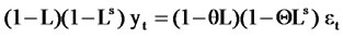 (1)
(1)
where L is the time lag (that is, the backshift) operator performing  and
and . Here, θ and
  are parameters that characterize respectively the non-seasonal and seasonal moving average (MA) components of the process. Further, the exponent s (on L) depicts the number of observations per year, and
  is a sequence of independent identically distributed (i.i.d.) set of random variables with
 , and
, and . The airline model is a member of the broader class of seasonal ARIMA models, which generalize the airline model formulation. Conventionally, in the relevant ARIMA pursuits, models are characterized by a set of parameters, namely, {autoregressive order, number of unit roots, moving average order} depicted identically as {(p, d, q) non-seasonal and (P, D, Q) seasonal}, and are specified by the following lag polynomial expression:
 (2)
(2)
where L, s and  are as in (1), the lag polynomials
  and
and  depict non-seasonal and seasonal autocorrelation (AR) filters, with orders p and P respectively. Further, the polynomials
  and
and  represent the non-seasonal and seasonal moving-average (MA) components, and are of order q and Q respectively. These polynomials generalize the parameters θ and
  of the airline model in (1). Lastly, d and D denote the orders of non-seasonal and seasonal differencing of the original series
 , respectively.
The airline model of Equation (1) can be obtained from the general formulation in (2) by setting p=0, P=0, d=1, D=1, q=1 and Q=1, that is, it is the seasonal ARIMA model {(0,1,1) (0, 1, 1) s}.
There are several alternatives to the airline model addressed in [7] (due to Findley et al.). They include more generalized airline models plus a restricted version known as the 1-12-13, which is used in the present work. It is specified in a convenient form in [9] as follows:
 (3)
(3)
where 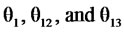 are the parameters of the model. Note that the airline model defined in Equation (1) corresponds to a restricted version of Equation (3), where
 ,
, , and
, and .
.
The ARIMA approach currently envisaged (following the Box-Jenkins model) decomposes the series into seasonal and non-seasonal parts and obtains the estimated time-series (which can be extended to forecast regime as well). The goodness-fit of such simplified models is then evaluated by applying some well-known criteria due to Akaike [10,11], and also validated in the frequencydomain [9]. Consideration is also given to the fact that these estimated models can be extended to the forecast regime as well.
5. Proposed Time-Series Analysis
The seasonal ARIMA model of Equation (2) is used to represent seasonal time series in the widely used forecasting software X12 [5] and TSW [12]. For a given data series, these programs can either estimate the coefficients of a given {(p, d, q); (P, D, Q)s} model chosen by the analyst, or be requested to choose the “best” seasonal ARIMA model from the set of all possible models. In the latter case the generalized model chosen is the one that shows a better adjustment to the series, when evaluated by a statistical metric such as Akaike Information Criterion (AIC) [10,11].
In typical use, this optimal choice of model is performed for an ensemble of time-series yielding several “best” models, one for each series of the data set. However, a cursory examination of the models chosen and represented by vectors {(p, d, q); (P, D, Q)s}, often indicates that the models that appear most frequently in yielding the “best” estimate constitute only a limited subset, as compared to the whole set of possible models. It follows that the analysis can be simplified by giving due consideration only to this restricted subset of “best” models. This selective adoption of models would significantly reduce computational burden that is otherwise imposed.
Hence, it is proposed in this work that it would suffice to identify and use only the models in this limited sense of subsets so as to get a good fit for the estimation. The models in this restricted set are further separated into two subsets of models: One comprises of non-seasonal models; and another of seasonal models. The choice of the subset in the analysis will be made for each time-series on the basis of a test for the presence/absence of the seasonal features.
In addition to the models selected by X12 and TSW, the 1-12-13 model is also included in the present work inasmuch as it is effective in signal extraction efforts as is evident in the models of economic series pertinent to several case studies tested by Findley et al. [7].
The selective option (of subsets) suggested above should, however, yield consistently an acceptable estimate of time-series that fits to the actual data set, regardless of the vagaries in the business structures to which the data belongs to. Hence, the underlying efficacy of the selective procedure should first be ascertained and confirmed, both time-and frequency-domain analyses. Relevant goodness of the estimation (of the time-series) is decided by the Akaike method [10,11]; and, the goodness-fit in frequency-domain is ascertained by computing the mean Euclidean distance between the actual frequency spectrum of the time-series (obtained via fast Fourier transform (FFT)) and the ARIMA-based estimates of the frequency spectrum.
5.1 Model Estimation
Model estimation steps are as follows (Figure 1):
Step 1: (a) The chosen telco economic test series are first transformed by taking logarithms so as to highlight the intrinsic properties of the time-series data. Relevant filtering or data-smoothing partially minimizes the computational burden due to outliers [13]; (b) also, in cases of extreme values typically observed with large amplitude fluctuations in the series [14], the logarithmic transformation smoothens out and stabilizes the variance; and, (c) the calculated mean of the transformed series (obtained as above) is then subtracted leading to “demeaning” of the log-transformed series.
Step 2: (a) The airline model (ARIMA (0, 1, 1) (0, 1, 1)), is fitted to each test time-series in the ensemble data set. When seasonality is present , the models being fitted to the series are chosen from the subset of seasonal models. Alternatively, if seasonality is absent
 , then the models are chosen from the subset
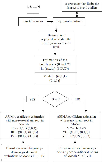
Figure 1. Flow-chart for the proposed estimation of ARIMA coefficients. (*Model V: corresponds to the 1-12-13 model of [7] where the set {(p, d, q); (P, D, Q)} is not used)
of non-seasonal models. That is, when  in Equation (1), the seasonal MA term in the right hand side cancels out the seasonal unit-root term in the left hand side, and the ARIMA process becomes a non-seasonal MA(1) process for the differenced series, namely,
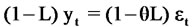 ; and, (b) this method of identifying the presence of a seasonal unit root is simpler than those traditionally available in the literature (due to Hylleberg et al. [15] and Frances [16] respectively).
Step 3: (a) Next the ensemble of time-series test-data is subjected to ARIMA modeling using the X12 [13] and TSW [19] programs so as to decide on the “best” model for each series; and, (b) from the collection of such optimally-decided ARIMA models, only a limited (five) subset (indicated as Models II, III, IV, VI, and VII in Figure 1) is chosen for subsequent use. The choice of five in the present study conforms to a set of two models having a seasonal unit root, and another set of three models that do not have a seasonal unit root. Additionally, the 1-12-13 model is also used (and designated as Model V in Figure 1).
Step 4: In this step, the ARIMA coefficients of the test-series for the models selected above are estimated. Relevant computation is done using the WinRats-7 time-series analysis software [17,18]. Models (in Step 3) with D=0 signify series that do not have a seasonal unit root, while models with  are for series that do have a seasonal unit root.
Step 5: In the time-domain, the goodness-fit of the estimation is evaluated by comparing the raw time-series (log-formatted and demeaned) with the time-series constructed with parameters obtained. The models fitted thereof should have a good adherence to actual time-domain data for any forecasting applications. The evaluation of the fit used here is based on the AIC of the Akaike method [10,11].
The frequency-domain goodness-fit of the model is evaluated by comparing the spectrum of the raw time-series to the frequency-spectrum of the corresponding ARIMA representation [19]. The spectrum of the raw data corresponds to the FFT transform of the given (raw) series, and the ARIMA-estimated spectrum is synthesized from the coefficients obtained. The fitted model should have a significant closeness to the raw data spectrum. Relevant evaluation is based on the calculation of an index equal to the sum over all frequencies of the absolute Euclidean distance between the FFT of the raw signal ARIMA-estimated spectrum.
5.2 Time-Domain Analysis
The test models are evaluated for their efficacy in time-domain in terms of the AIC. The lowest value of AIC indicates the “best estimate”. Specifically adopted in WinRats-7 software [17,18] is the formula for AIC given by: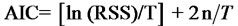 , where T is the number of observations along the time scale, n is the number of parameters estimated, and RSS is the residual sum-squared value, which refers to the sum of squared differences between the series,
 ,and its projected value,
 . That is,
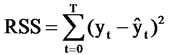 .
.
The calculations above are done for each of the test raw series, with an appropriate model (out of the seven indicated earlier). This is denoted by indexing the statistics as , where the subscripts i and m correspond to the raw series (i=1, 2, ..., I) and the model (m=1, 2, …, M=7) respectively. The index of average performance of (each model) in the time-domain can be calculated as the average AIC over all series fitted with that model. That is,
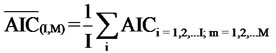 .
.
The test models of each category (with and without the seasonal unit root), is then compared in the time-domain on the basis of their average AIC. The goodness-fit in the time-domain can also be evaluated by comparing the plots of actual raw series (in log-demeaned format) and the corresponding series predicted by the ARIMA model, and also by evaluating the forecasting performance [5,12].
5.3 Frequency-Domain Analysis
For a given test series, the discrete spectrum is evaluated at (discrete) frequencies (given by , where k = 1,…, T) via Discrete Fourier Transform (DFT), namely,
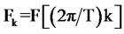 . The ARIMA-estimated power spectrum density
  is the square of the norm of the aforesaid discrete frequency response, given by:
 .
.
In order to compare the test models (Models I, etc.) of the present study, a statistical measure depicting the difference between them is indicated as the mean absolute deviation (MAD), which is calculated as follows:
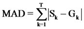 (4)
(4)
where  is the power spectrum density (PSD) of the data computed via Fast Fourier Transform (FFT) and
 , respectively. (Both Gk and Sk are expressed in dB). Further, the values of k corresponding to the seasonal frequencies are not included in the summation of Equation (9). Lastly, by indexing MAD as
 , with the subscripts i (= 1, 2, 3, …I) and m (=1, 2, 3, …M), each of the test series and the models is respectively designated. The average performance of each model in the frequency domain can be calculated by considering the average of all MAD values over the series fitted. That is,
  , where I (=8) is the total number of series that are fitted with model m. thus, the models of each category, (with and without seasonal unit root), can be compared in the frequency-domain on the basis of average MAD.
5.4 Combined Timeand Frequency-domain Analyses
The indicators of the performance via AIC and MAD in timeand frequency-domains (defined by Equations (4) and (10) respectively) can be linearly rescaled (normalized) between 0 and 1 and are denoted and
and . For either of these indices, the best performance corresponds to a value tending to zero, because it indicates the minimum absolute deviation in the timeand frequency-domains; and, a value of the indices tending to unity would correspond to the worst performance because it implies the largest deviation of the models selected over the series in the data set. Lastly, the two indices as above can be combined by their arithmetic average to produce an index of overall performance of each model. That is,
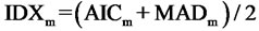 .
.
5.5 Merits of the Proposed Approach
The novelty of the proposed efforts can be observed by comparing the underlying considerations with those of existing methods. For example, the efforts in Hyndman et al. [20] do not include an upfront assertion as regards to knowing whether the data contains seasonal variations or not; and if the outcome on the computed time-series fail to give results to an expected level of accuracy, then the computation is redone (with the inclusion of seasonal attributes). Further, their computations refer only to a time-domain exercise with eventual goodness-fit done only in the time-domain. However, the goodness-fit of the series is verified in the present study, both in timeas well as in frequency-domain; hence it is more comprehensive in ascertaining the goodness-fit.
The present approach significantly pursues and extends the efforts due to Findley et al. [7] on the economic series pertinent to non-telco macroeconomic data. However, the differences in the levels of such estimations (in terms of accuracy) are not easily discernible because the seasonal component present is usually small in amplitude. Further evaluated in [9] is the efficacy of the generalized models in the frequency-domain with the introduction of a canonical seasonal adjustment filter, but without the adoption of a goodness-of-fit index done in the present approach.
According to [21], the simplified pre-selected use of a limited number of models was employed in pre-2000 versions of X12, but not in its current version [5]. The convenience of simplifying the models chosen by the automatic choice feature of the current version of X12 is indicated in [22], but has not been implemented.
6. Proposed Methodology: Implementation
In view of the above considerations and in concurrence with the views of Findley et al. [7], the present research is directed in applying the proposed method to the time evolutionary profiles of service growth data of modern telco enterprises. Essentially, the research effort pursued uses the available data specified in an ex post regime and the ex ante details of the technoeconomic growth are obtained. Determination of ex ante profile leads to forecasting feasibilities.
6.1 Description of the Telco Test Data
Few sets of seasonal data on telco services are readily available in the literature. From the published work, eight test time-series data (whose names and mnemonics are given in Table 1) are chosen as follows:
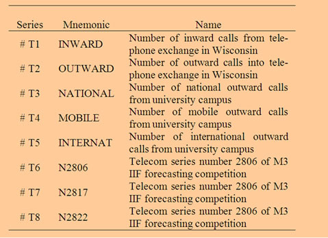
Table 1. Description of telco series (# T1 to # T8) test data
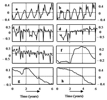
Figure 2. Plot of the demeaned and log-formatted telco series # T1 to # T8 shown as (a) through (h)
The two first Series (#T1 and #T2) report the number of incoming and outgoing telephone calls in an exchange of the Wisconsin Telephone Company, as reported by Thompson and Tiao [23]. This data has often been used to test telecommunications load forecasting models as, for example, by Madden et al. [24]. The test series considered display marked seasonal features, as well as clear technoeconomic time-trends.
The next three series (#T3 to #T5) refer to the number of outgoing calls of three types (national, mobile, and international) gathered at a university campus over a period of six years, and are available in [25].
The remaining three Series (#T6 to # T8) are from the dataset relevant to telco services and produced by the Institute of Forecasters for the M3 competition [26,27]. No explicit details on the underlying telco services are indicated in the data sources. They are simply identified by the codes N2806, N2817 and N2822 for those series [26]. A cursory examination of Figure 2, that displays the demeaned log transformed series, obtained as described earlier, indicates that telco Series # T2 to # T5 seem to exhibit a seasonal behavior, with the possible exception of 3, which displays irregular peaks and valleys. Series # T1, # T2 and # T4 have a clear time-trend, while the other seasonal series do not. The series # T6 to # T8, (extracted from the M3 IIF competition database), do not however, show any obvious seasonality et all. Series # T7 and # T8 have negative time trend, while Series # T6 has a peculiar behavior, namely, it is stable for the first 2 year, and then displays a “hump” in the last four years.
6.2 Selection of Models (I, II,…, VII)
In the seasonal ARIMA framework used here, the temporal trend is captured by the non-seasonal ARIMA parameters, while the seasonal ARIMA parameters capture the recurring time pattern. Consistent with this observation, both X12 and TSW programs choose as the “best” models for series 1 to 4 of the non-telco dataset those without a seasonal unit root with the vectors (1,1,1), (0,1,1) and (1,1,2) most frequently appearing in the non-seasonal part of these models. As such, these vectors are chosen as the non-seasonal specification of the Models II, III and IV and the seasonal part of those models is chosen as (0,0,0).
In all the chosen models, the seasonal part is seen to be the same as that of the airline model. Therefore, Models VI and VII, which have a seasonal unit root, also bear the same seasonal specification. For the non-seasonal part of these models, the vectors that appear most frequently are (1, 1, 2) and (2, 1, 1), and are therefore chosen as the non-seasonal specification of the Models VI and VII respectively.
6.3 Estimation of Seasonal ARIMA Coefficients
Consistent with Figure 1, first the procedures of log-transforming in demeaned format of the test data ensembles are performed. Then, the ARIMA coefficient estimation procedure of Model I (the airline model) is applied to the series and tested for the presence/absence of a seasonal unit root. Next, the ARIMA coefficients of the pertinent models are estimated with the software WinRats-7 [17,18].
The pseudocode of the procedure as above is presented Table 2. (The Box-Jenkins command is used with the option that allows for maximum-likelihood estimation because it enables more precise estimation than the alternative least-squares option).
6.4 Raw Data versus Estimated Models in Time-Domain
This section discusses the fitted and the original series in the time-domain making use of Series #T1 of the telco dataset as shown in Figure 3. A qualitative observation shows that for the test series, not only the airline model, but also its generalized versions appear to offer a good adherence to the raw data (inasmuch as no large deviations are observed across the broad stretches of their graphs). A small difference between the graphs of the
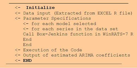
Table 2. Pseudocode: estimation of the ARIMA coefficients using WinRats-7
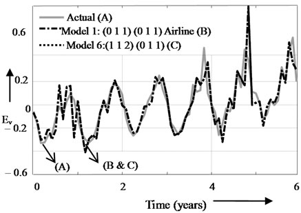
Figure 3. Actual and fitted values for demeaned and log-transformed data set of telco Series # T1 (Ev: Economic variable of interest normalized). (Note: The actual time-series data is shown as A and the computed model time-series data are indicated as B and C, which appear almost overlapping for the models pursued)
different models is however, observed for the other series of the dataset but within limits of acceptability of the goodness fit in the time-domain.
For quantitative model comparison, an indicator such as the quadratic-error adjusted for the different number of degrees of freedom encountered in different models, is needed. Hence, AIC mentioned earlier is used.
Another important dimension of goodness-of-fit in the time-domain refers to the forecasting performance. For this evaluation, the models of the series (of the telco database) are re-estimated excluding the end-section of nine months, respectively. With this exclusion, the data is considered as ex post data. And the forecasting is done in the period of last nine months taken as the ex ante regime. The forecast result is compared against the excluded data points. Relevant examples of such comparison are shown in Figure 4. They show a good forecasting performance of the estimated models.
6.5 Comparison of RAW Data and Estimated Models in the Frequency-Domain
Figure 5 shows the one-sided frequency-spectrum of the (demeaned and log-formatted) test series of telco data ensembles. These are obtained by calculating the discrete Fourier transform. The computation is performed through the FFT subroutine of MatLabTM. Examination of Figure 5 confirms the presence of seasonality, seen as peaks. The spectra of telco correspond to Series # (T1-T5). With the seasonal unit root ascertained, each series is conformed to an appropriate model designated earlier (as Models I to VII). The ARIMA-estimated spectrum is constructed for each series, and compared against the FFT-estimated spectrum. Examples of such comparisons are shown in Figure 6 for series #T1 of the telco dataset. The spectrum estimated by the airline model as well as the one estimated by the best extended airline model, are displayed.
In the estimated spectrum, the peaks occur at the frequencies that correspond to discrete locales (cycles per year) of the seasonal roots in the ARIMA models (I through VII), at the monthly, bi-monthly, quarterly, 4-month, half-year and yearly frequency. Only six peaks, rather than 12, appear in Figure 6 because they display the half-spectrum of the full spectrum symmetry.
As in the quarterly seasonal model above, there is also a peak at the zero frequency corresponding to the non-seasonal unit root. To a large extent, the models studies lead to estimated spectra that closely approximate the actual data spectra reproducing most of the peaks as in Figure 5. However, the symmetric nature of the unit roots in the seasonal ARIMA model imposes peaks at all integer seasonal frequencies, while the actual data do not display them for some frequencies. Also, in some cases, a peak exists in the actual spectrum for some frequencies, but does not have the intensity prescribed by the seasonal ARIMA model.
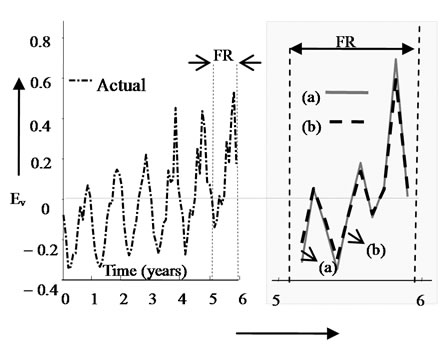
Figure 4. Time-series estimation in the forecast (ex ante) regime denoted as FR (3-steps ahead of last 9 months forecast based on demeaned log-transformed telco Series 1#T1 data). The forecast regime FR is shown with grey background expanded for clarity. (a) depicts Model 2: (1, 1, 1) (0, 0, 0) and (b) denotes Model 4: (1, 1, 2) (0, 0, 1). (Ev: Economic variable of interest normalized)
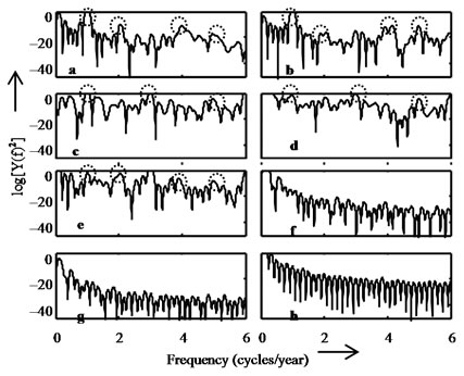
Figure 5. One-sided frequency spectrum: Demeaned and log-formatted telco series. (The encircled regimes denote some samples of explicit seasonal peaks)
6.6 Overall Performance with AIC and MAD
The relative values of AIC and MAD indices are presented in Figure 7 for telco datasets. In general, they show that the lowest value of the AIC (that indicates the best fit in the time-domain) is not necessarily compatible to the lowest value for the MAD index (depicting the best fit in the frequency-domain). Hence, an aggregation index can be specified by taking the mean of AIC and MAD indices as the overall goodness fit indicator in timeand frequency-domains.
Figure 7 shows, for example, that model VII namely, ARIMA (2, 1, 1) (0, 1, 1) is the best overall model for the Series # T1 and # T5 of the telco data set. In Figure 14, it can be observed that some series do not have values of AIC or MAD indices displayed for some models. This
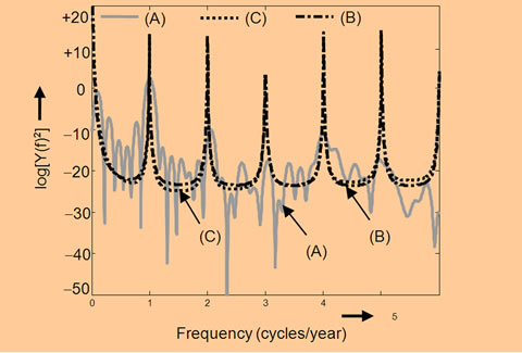
Figure 6. FFT and ARIMA power spectrum of the demeaned and log-formatted telco Series # T1 displaying distinct signature peaks. (A) depicts FFT estimation, (B) denotes Model 1: (0, 1, 1)(0, 1, 1)-Airline, and (C) corresponds to Model 6: (1, 1, 2)(0, 1, 1)
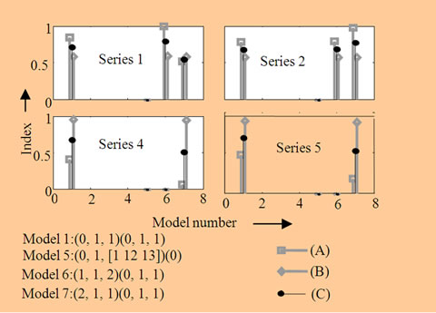
Figure 7. Normalized AIC and MAD indices of demeaned log-formatted telco series versus model number; (A) MAD of estimated power spectrum; (B) AIC of estimated time series; and (C) average of AIC and MAD
indicates that the estimation procedure does not converge for those cases. For example, it can be seen in Figure 14
Findley’s 1-12-13 model referred to Model 5 has not converged for any of the series in the telco dataset (that have a unit root).
7. Concluding Remarks
Telecommunications is viewed as a part of digital ecology with its underlying technoeconomics is analyzed via evolution considerations in terms of time-series. Hence, consistent with relevant procedure described in this paper, the following can be stated as closing remarks:
A simplified ARIMA-based time-series modeling of technoeconomic evolution in telecommunications (that display seasonal features) is feasible via the approach summarized as follows:
• A decision hypothesis is first projected to declare whether the data set is seasonal or not via the Box-Jenkins airline model. This avoids the complexity of pursuing computation with seasonal variation implications when seasonal attributes are absent. The use of the airline model for this purpose to the best of the authors’ knowledge is novel.
• The ARIMA-type models that characterize the seasonal and non-seasonal aspects of the time-series model are selected. The assertion above on the existence of seasonal and non-seasonal components leads to choosing the models to be estimated for the time-series from within two possible sets of models.
• In order to test the efficacy of the proposed methodology and to choose the “best” model, a comparison of estimated models versus real data is done in timeand frequency-domains. The criteria correspond to Akaike Information Criterion (AIC) and mean absolute deviation (MAD) metrics, respectively. They provide a dual assertion on the goodness-fit of the models for the time-series being evaluated. An aggregation index is specified by taking the mean of AIC and MAD indices to indicate the overall goodness-of-fit.
The usefulness of the proposed approach is ascertained in the present study by applying it to a diverse ensemble of time-series data of typical telco technoeconomics. The fitted models are compared with raw data in the timeand frequency-domains and their performance is assessed both in heuristic and quantitative terms summarized below:
• Examples of the heuristic assessment in both domains correspond to the inspection of graphs comparing the time-evolutions of the fitted and original series, and figures comparing the actual and fitted frequency spectra of some of the test series The models as chosen in this study provide a good fit for the data in both domains.
• Quantitatively assessment of AIC, MAD and their average confirms the selected model-based results offer good adherence to the raw data.
• The estimated models also lead to a good forecasting performance assessment for the test data.
In short, claimed here is that the proposed approach is computationally simple, enables an assured convergence of the series (regardless of the data set being intense or sparse) and the goodness fit of the estimation conforms to an acceptable extent both in timeand frequency domains. The efficacy of the proposal is demonstrated with real-world data sets concerning telco economics. Thus, the evolutionary aspect of a digital ecosystem is comprehended via time-series approach.
REFERENCES
- P. S. Neelakanta and R. Tourinho, “Modern/Next generation telecommunications—A digital ecosystem perspective in terms of complex system evolution,” Proceedings of 3rd IEEE International Conference on Digital Ecosystems and Technologies (IEEE DEST 2009), Istanbul, Turkey, pp. 441–446, 31 May–3 June 2009.
- P. S. Neelakanta and W. Deecharoenkul, “A complex system characterization of modern telecommunication systems,” Complex Systems, Vol. 12, pp. 31–69, 2000.
- P. S. Neelakanta and R. Tourinho, “Co-evolution of competitive businesses: A complex system model of technoeconomics in telecommunication service,” Complex System (under review).
- P. S. Neelakanta and D. Baeza, “Next generation telecommunications and Internet engineering,” Linus Publications, New York, 2009.
- U.S. Bureau of the Census, X-12-ARIMA Reference Manual (Final Version), Washington DC, 1999.
- G. Box and G. M. Jenkins, “Time series analysis: Forecasting and control,” Holden–Day, Oakland, 1976.
- D. F. Findley, D. E. K. Martin, and K. Wills, “Generalizations of the Box–Jenkins airline model,” Proceedings of the American Statistical Association, Business and Economic Statistics Section [CD–ROM], American Statistical Association, Alexandria, 2002.
- S. C. Hillmer and G. C. Tiao, “An ARIMA model–based approach to seasonal adjustment,” Journal of the American Statistical Association, Vol. 77, pp. 63–70, 2002.
- D. F. Findley and D. E. K. Martin, “Frequency domain analyses of SEATS and X-11/12-ARIMA seasonal adjustment filters for short and moderate-length time series,” Journal of Official Statistics, Vol. 22, No. 1, pp. 1–34, 2006.
- H. Akaike, “A new look at the statistical model identification,” IEEE Transactions on Automatic Control, Vol. 19, No. 6, pp. 716–723, 1974.
- H. Akaike, “Information theory and the extension of the maximum likelihood principle,” In: B. N. Petrov and F. Caaki, Eds., Second International Symposium on Information Theory, Budapest, 1973.
- G. Caporello and A. Maravall, “TSW—Revised reference manual,” mimeo, Banco de España, 2004.
- P. S. Neelakanta and A. Preechayasomboon, “Development of a neuroinference engine for ADSL modem applications in telecommunications using an ANN with fast computational ability,” Neurocomputing, Vol. 48, pp. 423–441, 2002.
- H. Lütkepohl and M. Krätzig, “Applied time series econometrics,” Cambridge University Press, New York, 2004.
- S. Hylleberg, R. F. Engle, C. W. J. Granger, and B. S. Yoo, “Seasonal integration and cointegration,” Journal of Econometrics, Vol. 44, pp. 215–238, 1990.
- P. H. Frances, “Testing for seasonal unit roots in monthly data,” Econometric Institute Report 9032A, Erasmus University, Rotterdam, 1990.
- Estima, “RATS version 7 reference manual,” Evanston, 2007.
- Estima, “RATS version 7 user guide,” Evanston, 2007.
- W. A. Gardner, “Statistical spectral analysis,” Prentice–Hall, Englewood Cliffs, 1988.
- R. J. Hyndman, A. B. Koehler, J. K. Ord, and R. Snyder, “Forecasting with exponential smoothing: The state space approach,” Springer–Verlag, Berlin, 2008.
- D. F. Findley and C. Hood, “X-12-ARIMA and its Application to Some Italian Indicator Series,” unpublished, 2000. http://www.census.gov/ts/papers/x12istat.pdf.
- K. M. McDonald–Johnson, C. H. Hood, and R. M. Feldpausch, “ Model simplification after the automatic modeling procedure of X-12-ARIMA Version 0.3,” Proceedings of the ASA 2004 Annual Meeting, American Statistical Association, November 2004.
- H. Thompson and G. Tiao, “Analysis of telephone data: A case study of forecasting seasonal time series,” Bell Journal of Economics and Management Science, RAND Corporation, Vol. 2, No. 2, pp. 515–541, 1971.
- G. S. Madden, J. Savage, and G. Coble-Neal, “Forecasting United States-Asia international message telephone service,” International Journal of Forecasting, Vol. 18, pp. 523–543, 2002.
- C. S. Hilas, S. K. Goudos, and J. N. Sahalos, “Seasonal decomposition and forecasting of telecommunication data: A comparative case study,” Technological Forecasting and Social Change, Vol. 73, pp. 495–509, 2006.
- “Database for the M3 competition,” International Institute of Forecasting, 2009. http://www.forecasters. org.
- S. Makridakis and M. Hibon, “The M3-Competition: results, conclusions and implications,” International Journal of Forecasting, Vol. 16, pp. 451–476, 2000.
- Census Data, 2008. http://www.census.gov.