Positioning
Vol.4 No.1(2013), Article ID:28383,15 pages DOI:10.4236/pos.2013.41006
A New Factorized Backprojection Algorithm for Stripmap Synthetic Aperture Radar
![]()
Microwave Earth Remote Sensing Laboratory, Brigham Young University, Provo, USA.
Email: moon@mers.byu.edu, long@ee.byu.edu
Received November 24th, 2012; revised December 25th, 2012; accepted January 8th, 2013
Keywords: Backprojection; Windows; Synthetic Aperture Radar (SAR)
ABSTRACT
Factorized backprojection is a processing algorithm for reconstructing images from data collected by synthetic aperture radar (SAR) systems. Factorized backprojection requires less computation than conventional time-domain backprojection with minimal loss in accuracy for straight-line motion. However, its implementation is not as straightforward as direct backprojection. This paper provides a new, easily parallelizable formulation of factorized backprojection designed for stripmap SAR data that includes a method of implementing an azimuth window as part of the factorized backprojection algorithm. We compare the performance of windowed factorized backprojection to direct backprojection for simulated and actual SAR data.
1. Introduction
Synthetic aperture radar (SAR) can generate high-resolution images from low-resolution data [1,2]. In stripmap SAR, a single antenna moving along a line is used to synthesize a linear array antenna, thus providing higher azimuth resolution than a single antenna position. Several algorithms have been proposed for image reconstruction of SAR data in both the time domain and frequency domain [3]. A particular time-domain algorithm known as backprojection is able to reconstruct well-focused images, even with non-ideal motion. Unfortunately, the computational complexity of backprojection is , which can quickly become computationally expensive.
Because of this computational cost, factorized backprojection was developed. This algorithm divides the process of backprojection into recursive steps to achieve complexity of . Factorized backprojection was first introduced by Rofheart and McCorkle [4] in the context of the quadtree, a data structure borrowed from computer science. The algorithm is designed so that the resolution improves by a factor of four each step.
Since then, multiple variations on factorized backprojection have been developed [2,5-11]. In particular, Ulander et al. [2] proposed a method called fast factorized backprojection, which uses the polar representation of an image to greatly reduce the number of operations. The factorized backprojection approaches assume constraints on the flight path, trading reduction computation for accuracy.
In this paper, we present a new formulation of factorized backprojection on a linear grid that does not use the polar representation and allows for easy parallelization of the algorithm. The method includes an azimuth window to reduce sidelobes and aliasing at a tradeoff in some loss in azimuth resolution. We compare performance of the windowed factorized backprojection algorithm with factorized and conventional time-domain backprojection.
The paper is organized as follows. Section 2 briefly reviews the time-domain backprojection. Section 3 provides an alternative derivation of factorized backprojection. Section 4 provides an error analysis of factorizedbackprojection. Section 5 introduces an azimuth window to the factorized backprojection algorithm. The results comparing the various algorithms are shown in Section 6.
2. Backprojection
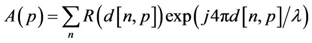
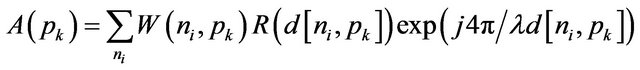
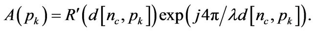
Backprojection is a time-domain algorithm that generates an image from SAR data. This process coherently integrates the radar data over each antenna position to form the image. Using the start-stop approximation, given a pixel at location p, the backprojected image  is given by [5,12]
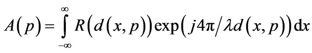 (1)
(1)
where  is the complex pixel value,
 ![]() is the wavelength of the transmit frequency,
is the wavelength of the transmit frequency,  is the distance between the pixel p and the along-track position x, and
  is the baseband range-compressed echo data interpolated to the distance
 . In practice, the echo data is digitized and a range window is applied. If we replace x with the discrete-time variable n representing the
  pulse, then this equation can be represented as
 (2)
(2)
where  is the distance between the antenna phase center of the
  pulse and the center of pixel p and
  is the range-compressed SAR data interpolated to slant range
 .
.
Although backprojection is straightforward to implement and can handle a variety of flight tracks, it can be computationally expensive. To obtain an image with M × N pixels from L equally spaced antenna pulse positions, a total of L × M × N square root calculations and transcendental computations must be performed. This can become costly as L, M, and N become large.
3. Factorized Backprojection Algorithm
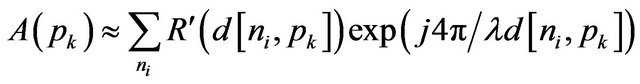
An alternative to direct backprojection is factorized backprojection. In factorized backprojection, the image reconstruction is divided into a series of steps in which the resolution of the image becomes finer as the length of a synthetic subaperture increases. The geometry of the SAR array allows the interpolated radar data associated with the subapertures of the previous step to be used in subsequent steps, reducing the required computation at a tradeoff of some loss of accuracy.
Although the formulation of factorized backprojection presented here uses recursive principles similar to the previous algorithms, there are some notable differences. First, this particular implementation is designed only for stripmap SAR. Like many previous implementations it uses the the start-stop approximation and assumes that the flight track is straight [2]. (For an explanation of the algorithm without the start-stop approximation, see [13]. The application of factorized backprojection to non-inear tracks is considered in [11,14]). Second, rather than divide the image into square subimages or use polar coordinates, the image is split into columns which are separately processed. In this paper, a column is defined as a one pixel wide region of the image in the range direction (see Figure 1). By splitting the image into columns, both the explanation and the implementation of the algorithm can be simplified. Additionally, the algorithm can be easily parallelized since each column can be formed independent of the others.
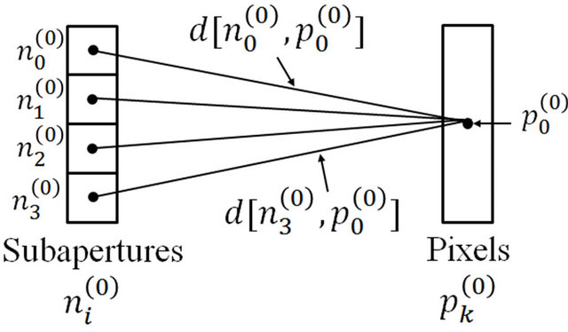
We now describe this factorized backprojection algorithm in detail. Suppose there are L collected pulses with which we wish to image an area comprised of M × N
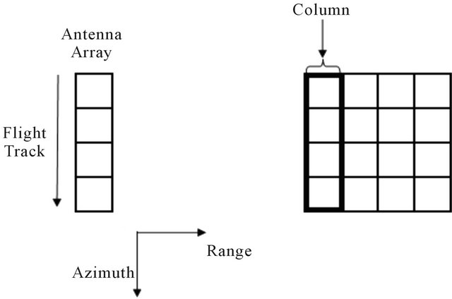
Figure 1. Left: Notional antenna phase center positions. Each position corresponds to the antenna location for a transmit/receive pulse. Right: Imaging grid with a single column highlighted.
pixels. Then, the number of stages is min{log2L, log2M}, in addition to a preliminary stage. For this explanation, we assume L = M = N = 4 and that the pulses and pixels are equally spaced. In practice, however, L, M, and N do not need to be equal, nor do the pulses and pixels need to be equally spaced. We note that a pixel must lie in the beamwidth of the real aperture to be fully reconstructed. For pixels on the edge of an image, reconstruction requires antenna positions that extend beyond the imaging grid.
Initially, each subaperture corresponds to the actual antenna positions for each collected pulse, but in later steps it corresponds to the combination of two or more adjacent antenna positions. We divide the image into subimages, or sections of columns. Initially, a subimage consists of a single large area covering the entire column, but by the final stage, each of the multiple subimages is a single pixel of the column. (To reduce error, a subimage may initially consist of a portion of a column rather than the entire column, but this increases the total number of computations despite decreasing the number of steps). Because the same algorithm is applied for each column independent of the other columns, we concentrate on a single column in this explanation.
Since the central positions of both subimages and pulses change for each step of the factorization, we introduce some notation to aid in the explanation. Let  index the center of the
  pulse on the
  step. Let
  index the center of the
  subimage on the
  step in the along track direction. The distance from the
  subaperture center to the
  subimage is denoted
  and the interpolated range-compressed complex SAR data set associated with this subaperturesubimage pair is denoted
 . In the preliminary step, the data set is the range-compressed SAR data interpolated to slant range, but in subsequent steps the data set is formed from combinations of elements from the parent data set.
In the preliminary step of the algorithm, the distance from each subaperture center (pulse) to a subimage center is calculated. Since our example involves four pulses and one initial subimage, this step requires four distance calculations. In Figure 1, which shows the preliminary step of the algorithm, the central pixel is denoted , and each pulse is denoted as
 ,
, . Once each distance
  has been calculated, the radar echo data
  is found from the rangecompressed SAR data.
For the first factorization step, the number of subapertures is decreased by a factor of two by combining the parent subapertures into longer child subapertures. Because the resulting subapertures are longer than the parent subapertures, the corresponding beamwidth is narrower. In addition, the subimage is divided in half so that there are two pixels per column rather than one (see Figure 1).
The distance from each subaperture center  to each subimage center
  is calculated, where
  has coordinates
  and
and  has coordinates
 . Then, the distance from each parent subaperture center
  to each subimage center
  is calculated or approximated. Given a parent subaperture
  with coordinates
 , the distance from
  to the
  subimage center is given by
 (3)
(3)
If the flight track is parallel to the image column and the imaging area is flat, then the distance can be approximated using a Taylor series approximation:
 (4)
(4)
where
 (5)
(5)
(see Figure 1). Note that for our column-based algorithm with a flat surface, 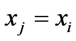 and
and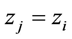 .
.
Because the child subapertures are longer than the original subapertures, there is no previously interpolated radar data corresponding exactly to these new subapertures. However, we can construct data sets  corresponding to these longer subapertures by combining the data sets from parent subapertures and multiplying by a phase factor to compensate for the difference in distances:
 (6)
(6)
where
 (7)
(7)
or if the prior distances are calculated with a Taylor series approximation,
 (8)
(8)
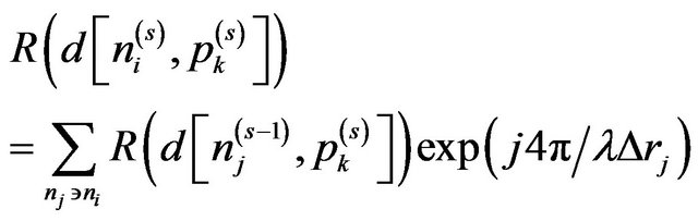
Rather than directly calculating , to save computation we approximate it from values computed in the previous step, i.e.,
 (9)
(9)
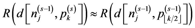
If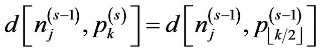 , there is no error in the approximation. However, if the distances are not equal, the approximation may not correspond to the same range bin as the correct data value. This adversely impacts the image focusing since the incorrect phase may be computed in Equation (6). We discuss these errors more in Section 4.
For the remaining iterations, the process of lengthening subapertures and decreasing subimage size continues until a subimage is a single pixel and there is only one subaperture covering the full synthetic aperture with center  (see Figures 2(d) and (e)). The reconstructed pixel
  at the final subaperture level is given by
 (10)
(10)
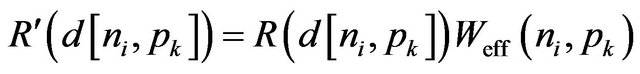
4. Errors in the Factorized Backprojection Algorithm
Two types of errors are associated with factorized backprojection in the scenario considered: those caused by errors in the creation of data sets from the range interpolated data, and those caused by using incorrect distances for phase calculations due to the factorization. Note that in a realistic scenario, deviations of the platform from its ideal path introduce variations in the desired phase for image formation.
Recall that in the creation of the data set  , we make the approximation
 (11)
(11)
That is, we assume that the radar data associated with a given subaperture and subimage is the same as the radar data associated with the subaperture and the parent subimage. Since data is considered constant over a range bin, this assumption is true so long as both subimages lie within the same range bin. However, if both subimages do not lie in the same range bin, then the data corresponding to the child subimage is from the wrong range
 (a)
(a)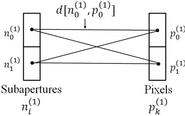 (b)
(b)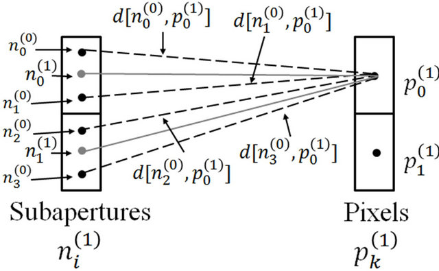 (c)
(c)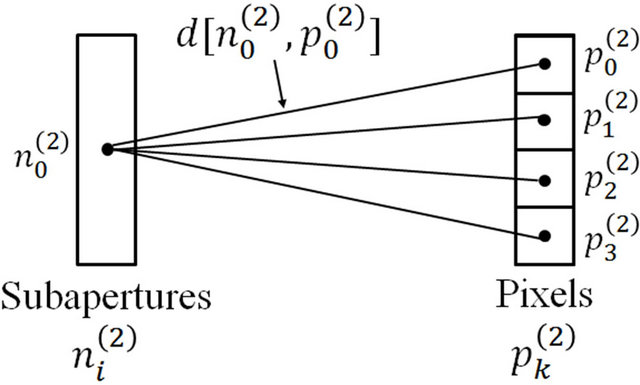 (d)
(d)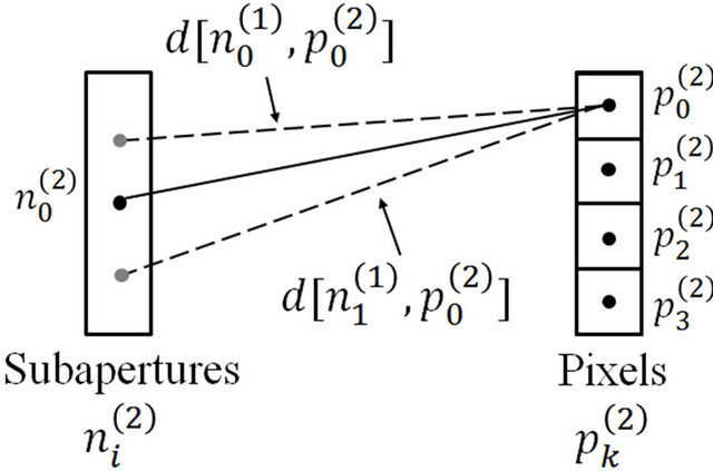 (e)
(e)
Figure 2. Illustration of distance calculations for factorized backprojection algorithm (see text). (a) Distance from current subaperture centers to current subimage centers for preliminary step; (b) Distance from current subaperture centers to current subimage centers for first step; (c) Distance from parent subaperture centers to current subimage centers for first step; (d) Distance from current subaperture centers to current subimage centers for second step; (e) Distance from parent subaperture centers to current subimage centers for second step.
bin, causing errors. We can avoid these errors by requiring that the range migration be limited to a range bin. Although an image can be reconstructed with some error when the range-cell migration spans multiple range bins, we do not address this case here.
The other type of error in factorized backprojection is the phase error caused by not directly calculating 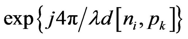 for each pulse
  and pixel
  and instead using an approximation formed over a series of steps. The effective phase term for a given pulse
  and pixel
  is of the form
  where
where
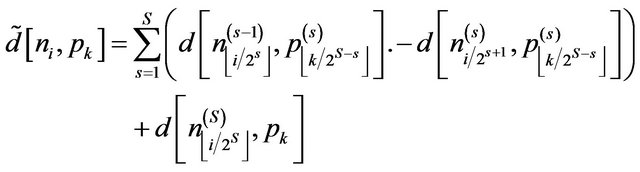 (12)
(12)
For convenience we refer to  as the factorized distance as the distance used by the factorized backprojection to discriminate it from the actual distance. Ideally, the actual distance
  equals the factorized distance. However, in practice, this is not generally true. We can obtain an upper bound on the error by setting a single pixel and pulse as reference points and then defining the coordinates of the parent subimages and child subapertures in terms of these reference points.
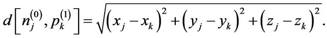
Let a pixel  have coordinates
  and let a pulse
  have coordinates
 , where the azimuth direction is in
![]() . Let
. Let  be the length of the imaging grid,
  be the number of pixels in the imaging grid,
  be the length of the antenna array, and
  be the number of pulses. Let
  be the minimum distance from the SAR array to the column. Let
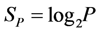 ,
,  , and
, and . Then, a parent subimage center
  has coordinates
 , where
 (13)
(13)
Similarly, a child subaperture center 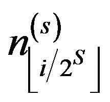 has coordinates
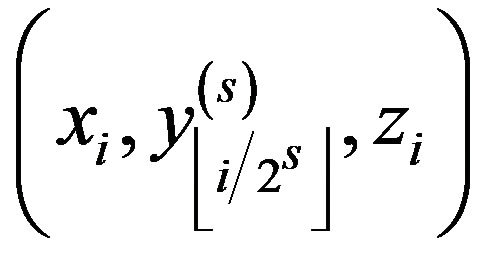 , where
 (14)
(14)
Let 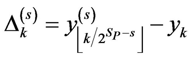 and
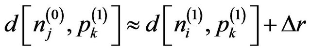
and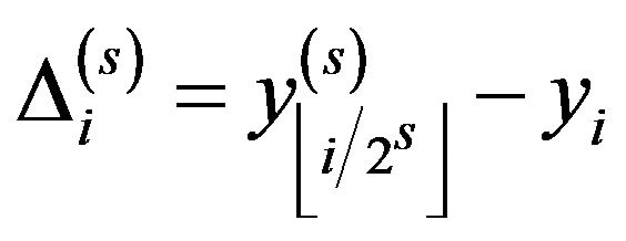 . Using these relationships, the error
 ![]() between the actual distance and the factorized distance from a pulse
between the actual distance and the factorized distance from a pulse  and a pixel
  can be written as
 (15)
(15)
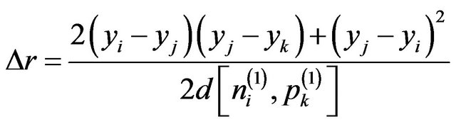
We can approximate ![]() by
by , where
 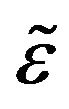 is the Taylor series approximation given by
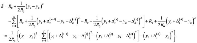 (16)
(16)
By canceling and rearranging terms, this equation can be further simplified as
 (17)
(17)
We note that
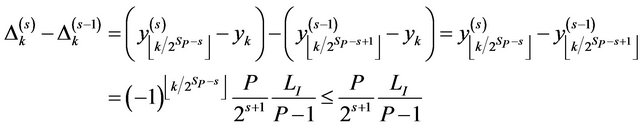 (18)
(18)
Thus,
 (19)
(19)
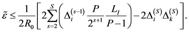
Using the triangle inequality, we can further bound Equation (17) by
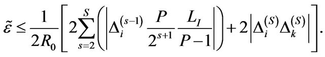 (20)
(20)
Since for any given pulse ,
,
and for any given pixel ,
,
we can further simplify the bound in Equation (20) as
 (21)
(21)
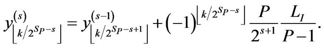
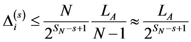
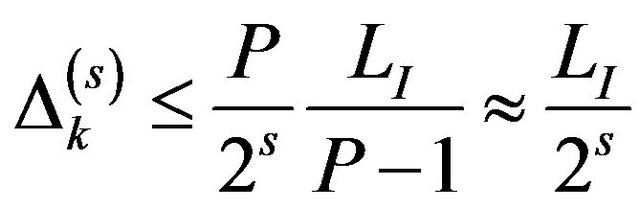
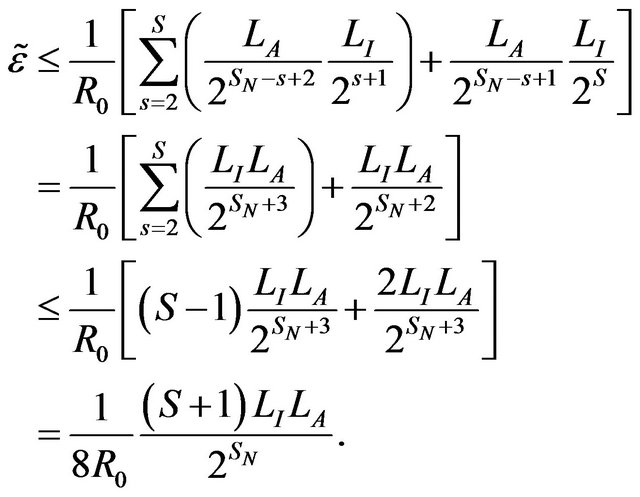
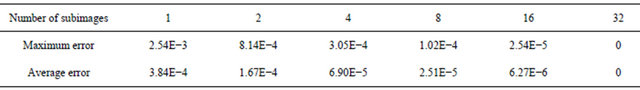
Note the similarity of this error bound to that given by [2]. From this equation, we see that the distance error can be reduced by decreasing the length of the image to be reconstructed. Similarly, by initially dividing a column into several subimages rather than performing factorized backprojection for the entire column, the error is reduced because each subimage is shorter, reducing . However, this requires more computation. Table 1 shows the distance error for simulated data for a given pixel and varying numbers of initial subimages for a 64 by 64 grid of pixels. As the number of initial subimages increases, the error is reduced. Note that for the initial subimages, the phase error is zero because each distance is calculated correctly in the algorithm.
Recall that ![]() is the difference between the actual distance and factorized distance for a given pulse and pixel. A commonly assumed value for the acceptable phase error is
is the difference between the actual distance and factorized distance for a given pulse and pixel. A commonly assumed value for the acceptable phase error is 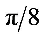 [1], though the precise value is not critical for our analysis. Using this value, there is negligible error in the image if
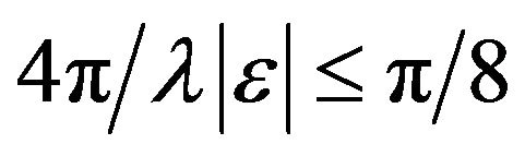 (22)
(22)
which implies
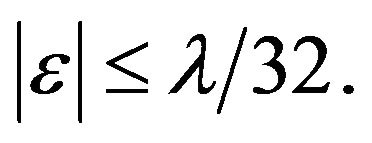 (23)
(23)
For the simulation described in Section 6 with average and maximum error ishown in Table 1, the wavelength of the transmit frequency is 0.0292 m, so λ/32 = 9.1250 × 10⁻⁴. In Table 1, the bound on the distance error is less than this when more than one initial subimage is used.
5. Windowed Factorized Backprojection
In SAR image processing, an azimuth window is often applied to minimize azimuth aliasing and suppress sidelobes at a cost of some loss in azimuth resolution. In this section, we show that an azimuth window can also be incorporated into our factorized backprojection with little additional computation.
Table 1. Error between actual and factorized distances for each pixel within a column and each pulse in the antenna array for the parameters in Table 2.
For direct backprojection, if an azimuth window is desired for some pixel , one approach is to apply a weighting function to the backprojection equation:
 (24)
(24)
where  is a weighting function expressed in terms of the pulse number
  and specified pixel
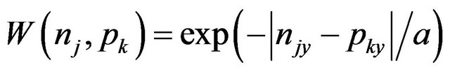
 . In this paper we consider weighting functions of the form
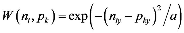 (25)
(25)
where  is the y-coordinate of
 ,
,  is the y-coordinate of
 , a is some constant, and the azimuth direction is in y. The output of the weighting function for a given pixel p is a Gaussian curve, thus creating a window for the given pixel. We call this the direct window.
In factorized backprojection, implementing an azimuth window is more complex because the algorithm is divided into a series of steps. Since there is no single equation that depends on both an individual pulse  and an individual pixel
 , there is no place where the weighting term
  used in direct backprojection can be logically inserted. However, an alternative approach is to include intermediate weighting functions in the formation of the data sets for each step to create windowed data sets
 . Then, in the final step of windowed factorized backprojection, the equation for a pixel
  takes the form
 (26)
(26)
If 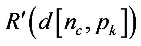 is written in terms of its parent data sets, then
 (27)
(27)
where
 (28)
(28)
where  is the effective weighting function formed in the steps of the algorithm corresponding to a pulse
  and a pixel
 . We call the output of this weighting function the factorized window. Due to the factorization, the factorized window is not identical to the direct window. However, by the proper choice of intermediate weighting functions, the factorized window can be similar to the direct window.
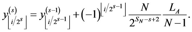
We now discuss an intermediate weighting function that is easy to implement and which creates a factorized window that is similar to the direct window. Consider an intermediate subaperture center  with parent subaperture center
  with coordinates
  and an intermediate subimage center
  with coordinates
 . We define an intermediate weighting function
 to weight the corresponding data set as
 (29)
(29)
where
 (30)
(30)
with a determined as a function of the beamwidth. Given a pulse  and a pixel
 , the resulting effective weighting function corresponding to
  and
and  is
is
 (31)
(31)
Figure 3 plots the factorized window and direct window for given pixels located in various locations of an imaging grid. Note that the shape of the factorized window is similar to the shape of the direct window for each pixel. However, while the direct window has the same shape regardless of the pixel, the factorized window changes shape slightly for different pixels. This discrepancy is expected due to the creation of the window over a
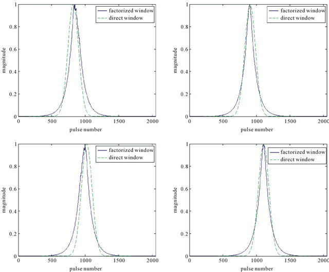
Figure 3. Effective factorized and actual weighting functions for various pixels in a column of 64 pixels. Upper left: pixel 1; upper right: pixel 14; lower left: pixel 32; lower right: pixel 45.
series of steps.
6. Performance Evaluation
In this section we display images formed by factorized and windowed factorized backprojection and compare them to images formed with direct backprojection. We consider both simulated and actual data. Note that because factorized backprojection is not exact, we expect some performance degradation compared to backprojection, particularly for non-ideal motion. Also note that we did not attempt to optimize the impulse response function, though techniques to accomplish this are given in [15].
6.1. Results for an Ideal Track
We first assume that the flight track is ideal, that is, straight and level, with uniform spacing. Figure 4 shows the impulse response (IPR) of a point target created with noise-free simulated data acquired from an L-band pulsed SAR (parameters given in Table 2) which was reconstructed with direct backprojection. Figure 5 shows the IPR of the same point target reconstructed with factorized backprojection. Note that both images have notable azimuth sidelobes.
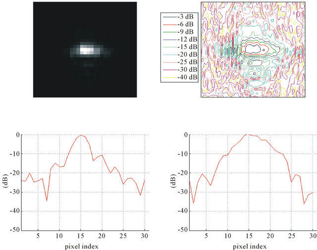
When a window is added to the direct backprojection image, the image quality improves, although the resolution is slightly degraded as evidenced by the wider target main lobe (see Figure 6). When the window is applied to the factorized backprojection image, the image improves, although with similar resolution loss. Figure 7 shows the windowed factorized backprojection image where each pixel has been normalized by the area of the effective window on the pixel. Note that the width of the main lobe in the azimuth direction for both windowed images is slightly wider, resulting in slightly coarser resolution. However, the sidelobes have been reduced considerably
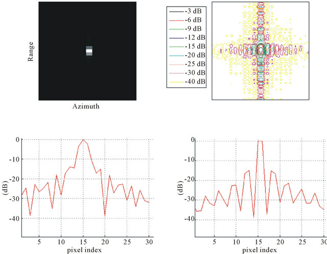
Figure 4. Point target IPR from simulated SAR data collected on an ideal track with parameters given in Table 2 using direct backprojection. Upper left: power image (linear scale); upper right: contour plot; lower left: range slice through peak; lower right: azimuth slice through peak.
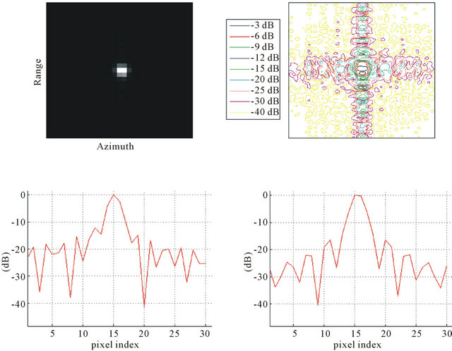
Figure 5. Point target IPR from simulated SAR data collected on an ideal track with parameters given in Table 2 using factorized backprojection. See caption for Figure 4.
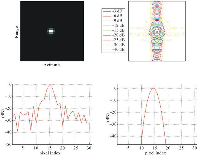
Figure 6. Point target IPR from simulated SAR data collected on an ideal track with parameters given in Table 2 using direct backprojection with a Gaussian window. See caption for Figure 4.
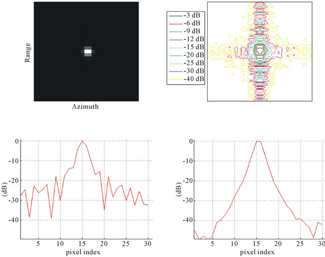
Figure 7. Point target IPR from simulated SAR data collected on an ideal track with parameters given in Table 2 using factorized backprojection with a factorized window. See caption for Figure 4.
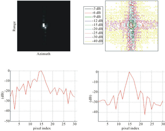
Figure 8. Point target IPR from simulated SAR data collected on a non-ideal track with parameters given in Table 2 using direct backprojection. See caption for Figure 4.
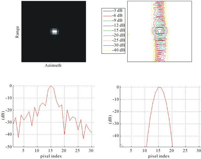
Figure 9. Point target IPR from simulated SAR data collected on a non-ideal track described in the text with parameters given in Table 2 using direct backprojection with a Gaussian window. See caption for Figure 4.
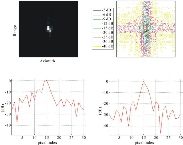
Figure 10. Point target IPR from simulated SAR data collected on a non-ideal track described in the text with parameters given in Table 2 using factorized backprojection. See caption for Figure 4.
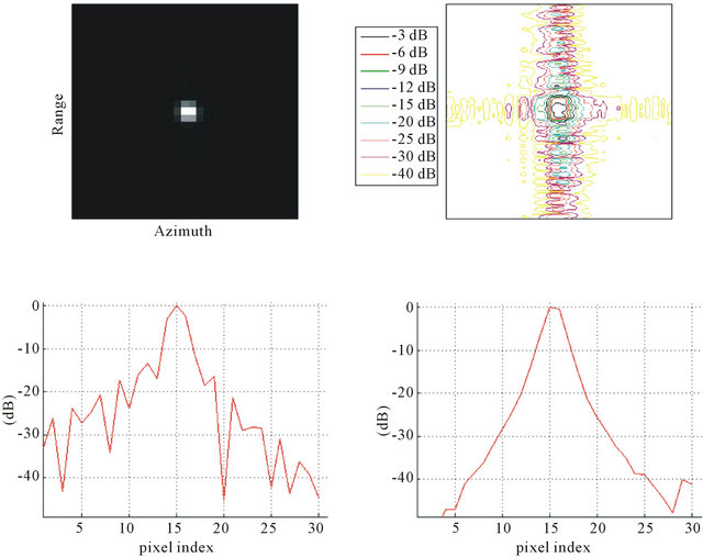
Figure 11. Point target IPR from simulated SAR data collected on a non-ideal track described in the text with parameters given in Table 2 using factorized backprojection with a factorized window. See caption for Figure 4.
 (a)
(a)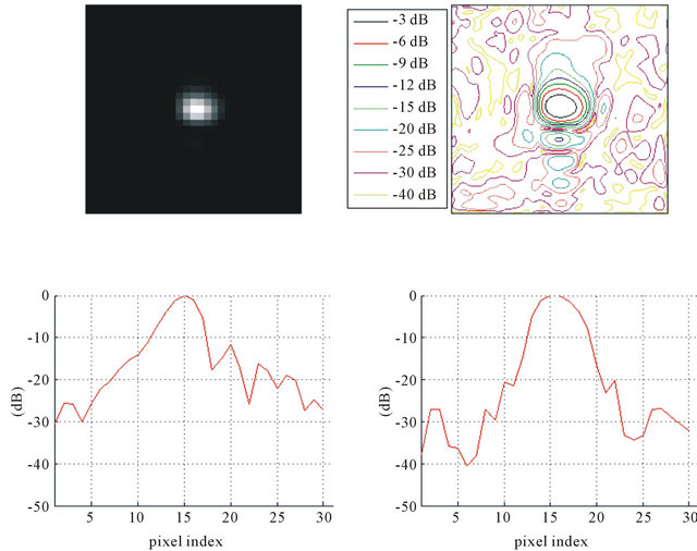 (b)
(b)
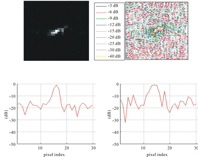
Figure 12. Images generated from real SAR data of uniform scene with a trihedral corner reflector. Note there is real (and hence non-ideal) unknown motion of the SAR. Parameters given in Table 3. (a) IPR response of corner reflector in direct backprojection image; (b) IPR response of corner reflector in factorized backprojection image.
 (a)
(a)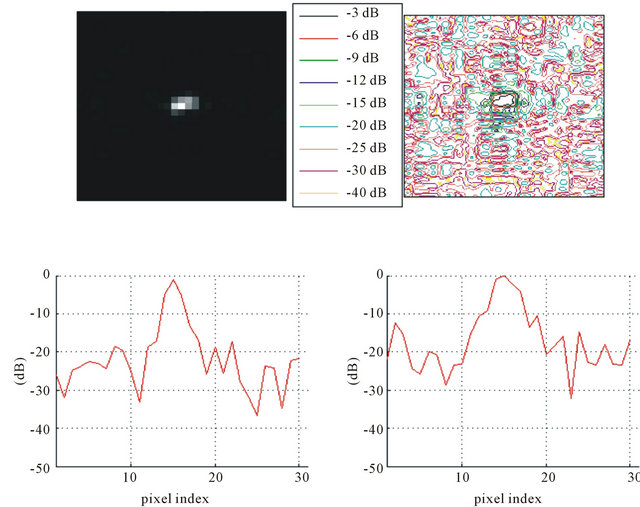 (b)
(b)
Figure 13. Images generated from real SAR data of uniform scene with a trihedral corner reflector. Note there is real (and hence non-ideal) unknown motion of the SAR. Parameters given in Table 3. (a) IPR response of corner reflector in windowed direct backprojection image; (b) IPR response of corner reflector in windowed factorized backprojection image.
in Figures 5-7.
6.2. Results on a Non-Ideal Track
If the flight track is non-ideal, then factorized backprojection becomes less accurate because the range bins corresponding to a child subaperture may differ from the range bins corresponding to a parent subaperture (see [2] for a more complete analysis). To illustrate this, we simulated a non-ideal flight track with a sinusoidal movement at an amplitude of 1 m (which spans more than one range bin). In Figures 8-11, the IPR is shown when the flight track is non-ideal for an image reconstructed with direct, windowed direct, factorized, and windowed factorized backprojection, respectively. As expected, the performance of the factorized backprojection is degraded compared to full backprojection for a non-ideal track. However, including the window improves the image. Further research is needed to quantify the level of improvement provided by the window for factorized backprojection on a non-ideal track.
6.3. Results with Real Data
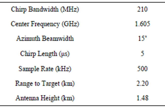
Figures 12 and 13 shows various images generated from real SAR data of a uniform scene with a trihedral corner reflector (parameters given in Table 3). There are 4096 aperture positions and an image grid of 1024 × 1024 pixels, with each pixel 0.5 m by 0.3 m. Figure 12(a) shows the results of direct backprojection, and Figure 13(a) shows the results with windowed direct backprojection. Figure 12(b) shows the same image reconstructed using
Table 2. Summary of simulation processing parameters for Figures 4-11.
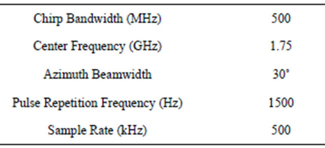
Table 3. Summary of processing parameters for Figure 12.
factorized backprojection. Note that the corner reflector appears more smeared in the factorized backprojection image than in the direct backprojection image, mostly due to non-ideal motion. Figure 13(b) shows the image reconstructed with windowed factorized backprojection. Note the improvement of the IPR response when a window is added to factorized backprojection.
7. Conclusions
In this paper, a new formulation of factorized backprojection is introduced. A new algorithm to incorporate an azimuth window is described, termed windowed factorized backprojection. Unlike previous formulations of factorized backprojection, this algorithm divides an image into columns parallel to the flight track rather than into quadtrees. This feature of the algorithm aids in the parallelization of the algorithm and enables the easy addition of a factorized azimuth window by introducing intermediate windows in each step. Errors are introduced into the image due to a combination of range errors and range-cell migration but can be minimized by dividing an image into subimages of shorter length and backprojecting each independently.
The performance of windowed factorized backprojection is verified with simulated and real SAR data. The performance of windowed factorized backprojection on non-ideal flight tracks is briefly examined, and it is shown that windowed factorized backprojection can handle some non-ideal tracks. As expected, compared to direct backprojection, the performance is not as good but requires less computation. No attempt was made to optimize the windowing, but rather a basic window was introduced which was independent of the data. However, such optimization could further improve the algorithm.
REFERENCES
- C. Elachi, “Spaceborne Radar Remote Sensing: Applications and Techniques,” IEEE Press, New York, 1988, pp. 72–77.
- L. Ulander, H. Hellsen and G. Stenstrom, “Synthetic Aperture Radar Processing Using Fast Factorized BackProjection,” IEEE Transactions on Aerospace and Electronic Systems, Vol. 39, No. 3, 2003, pp. 760-776. doi:10.1109/TAES.2003.1238734
- I. Cumming and F. Wong, “Digital Processing of Synthetic Aperture Radar Data,” Artech House, Norwood, 2005.
- M. Rofheart and J. McCorkle, “An Order N2 log N Backprojection Algorithm for Focusing Wide Angle Wide Bandwidth Arbitrary-Motion Synthetic Aperture Radar,” SPIE Radar Sensor Technology Conference Proceedings, Orlando, 8 April 1996, pp. 25-36.
- A. Hunter, M. Hayes and P. Gough, “A Comparison of Fast Factorised Back-Projection and Wavenumber Algorithms,” Fifth World Congress on Ultrasonics, Paris, 7-10 September 2003, pp. 527-530.
- S. Oh and J. McClellan, “Multiresolution Imaging with Quadtree Backprojection,” 35th Asilomar Conference on Signals, Systems and Computers, Pacific Grove, 4-7 January 2001, pp. 105-109.
- S. Basu and Y. Bresler, “
 Filtered Backprojection Reconstruction Algorithm for Tomography,” IEEE Transactions on Image Processing, Vol. 9, No. 10, 2000, pp. 1760-1773. doi:10.1109/83.869187
 - H. Callow and R. Hansen, “Fast Factorized Back Projection for Synthetic Aperture Imaging and Wide-Beam Motion Compensation,” Proceedings of the Institute of Acoustics, Vol. 28, 2006, pp. 191-200.
- J. Xiong, J. Chen, Y. Huang, J. Yang, Y. Fan and Y. Pi, “Analysis and Improvement of a Fast Backprojection Algorithm for Stripmap Bistatic SAR Imaging,” 7th European Conference on Synthetic Aperture Radar (EUSAR), June 2008, pp. 1-4.
- S. Xiao, D. C. Munson, S. Basu and Y. Bresler, “An N2logN Back-Projection Algorithm for SAR Image Formation,” Proceedings of the 34th Asilomar Conference on Signals, Systems and Computers, Pacific Grove, 29 October-1 November 2000, pp. 3-7.
- M. Rodriguez-Cassola, P. Prats, G. Krieger and A. Moreira, “Efficient Time-Domain Image Formation with Precise Topography Accommodation for General Bistatic Sar Configurations,” IEEE Transactions on Aerospace and Electronic Systems, Vol. 47, No. 4, 2011, pp. 2949- 2966. doi:10.1109/TAES.2011.6034676
- A. Ribalta, “Time-Domain Reconstruction Algorithms for FMCW-SAR,” IEEE Geoscience and Remote Sensing Letters, Vol. 8, No. 3, 2011, pp. 396-400. doi:10.1109/LGRS.2010.2078486
- K. M. Moon, “Windowed Factorized Backprojection for Pulsed and LFM-CW SAR,” Master’s Thesis, Brigham Young University, Provo, 2012.
- M. Brandfass and L. Lobianco, “Modified Fast Factorized Backprojection as Applied to X-Band Data for Curved Flight Paths,” 7th European Conference on Synthetic Aperture Radar (EUSAR), June 2008.
- L. Ulander and P. Frolind, “Evaluation of Angular Interpolation Kernels in Fast Back-Projection SAR Processing,” IEE Proceedings on Radar, Sonar, and Navigation, Vol. 153, No. 3, 2006, pp. 243-249.
Appendix
SAR Parameters
This section contains tables with the processing parameters for both the simulated and real SAR data used in Section 6. The parameters for simulated data are shown in Table 2, and the parameters for real data are shown in Table 3.