Natural Science
Vol.5 No.4(2013), Article ID:29936,17 pages DOI:10.4236/ns.2013.54061
Solution of non-linear boundary value problems in immobilized glucoamylase kinetics
![]()
1Department of Mathematics, Ganesar College of Arts and Science, Melaisivapuri, India
2Department of Mathematics, K. L. N. College of Engineering, Pottapalayam, India
3Department of Mathematics, The Madura College, Madurai, India; *Corresponding Author: raj_sms@rediffmail.com
Copyright © 2013 Swaminathan Sevukaperumal et al. This is an open access article distributed under the Creative Commons Attribution License, which permits unrestricted use, distribution, and reproduction in any medium, provided the original work is properly cited.
Received 25 December 2012; revised 27 January 2013; accepted 10 February 2013
Keywords: Reaction-Diffusion System; Immobilized Enzyme; Adomian Decomposition Method; Homotopy Analysis Method; Boundary Value Problems
ABSTRACT
A mathematical model to describe the enzyme reaction, mass transfer and heat effects in the calorimetric system is discussed. The model is based on non-stationary diffusion Equation containing a non-linear term related to immobilize liver esterase by flow calorimetry. This paper presents the complex numerical methods (Adomian decomposition method, Homotopy analysis and perturbation method) to solve the nonlinear differential Equations that depict the diffusion coupled with a non-linear reaction terms. Approximate analytical expressions for substrate concentration have been derived for all values of parameters α, β and γE. These analytical results are compared with the available numerical results and are found to be in good agreement.
1. INTRODUCTION
Flow reaction calorimetry has several advantages over a batch calorimetry method. The operation at a calorimetric experiment can be made exceedingly simple and equilibration time prior to the experiment can be omitted. Mixing of reactants can be achieved without the presence of a gaseous phase which is of great importance when experiments are performed with volatile liquids and in micro-calorimetric expriments where very small condensation-evaporation effects may affect the result. Surface adsorption effects which may cause seious systematic errors in micro calorimetry can be neglected if a steady liquid flow is allowed to continue until possible wall reactions have occurred [1]. Immobilized biocatalysts (IMB)- enzymes or whole cells are used in various areas of analytical, medical, and industrial applications. Basically, enzyme kinetic parameters cannot be determined experimental data. For this purpose many experimental techniques can be used, that are more or less laborious and time consuming. Reaction kinetics of carboxyl esterase’s depends strongly on the nature of substrate. The hydrolysis of different substrate activation [2] or it can follow the simple Michaelis-Menten kinetics [3].
Stefuca et al. [4] have described the principles and applications of flow calorimetry (FC) in the investigation of the IMB properties. One of the last improvements of this technique was the introduction of an “auto calibration” principle based on reaction solution recirculation enabling to determine true reaction rate of biocatalyst reaction without any requirement of an additional analytical technique [5]. Vladimir Stefuca et al. [6] have derived the experimental data were treated by mathematical modelling based on material and heat balances of the reaction system. Recently, Fedor Malik [7] has developed the mathematical model describing the enzyme reaction, mass transfer and heat effects in the calorimetric system.
To my knowledge no rigorous analytical solutions of the substrate of phenyl acetate hydrolysis with steadystate conditions for all values of parameters  and
and  have been reported. The purpose of this communication is to derive approximate analytical expressions for the steady-state concentration of substrate using Adomian decomposition method, Homotopy analysis and perturbation method.
2. MATHEMATICAL FORMULATION OF THE PROBLEM
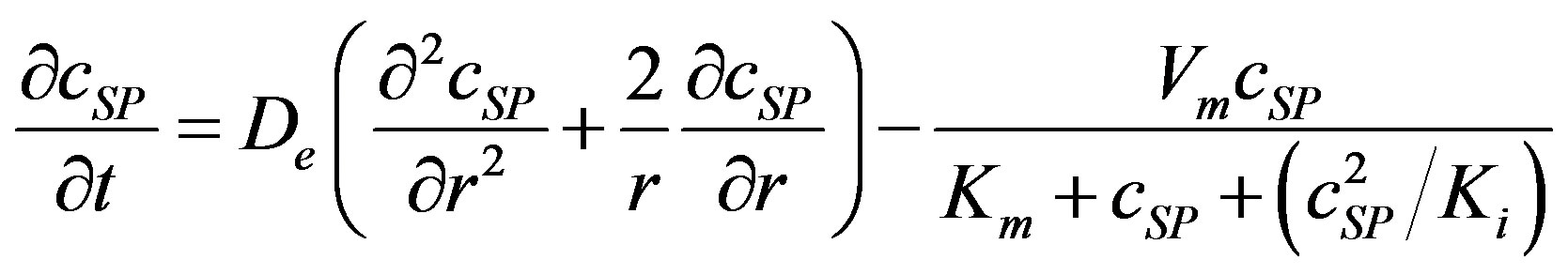
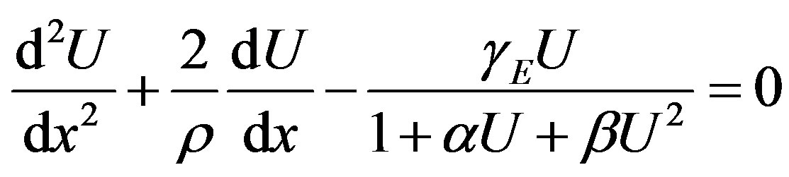
The experimental set-up used for the capacity is depicted in (Figure 1). The main part of the system thermostatic cell through immobilized enzyme column. The column was operated packed bed reactor The temperature difference between the column input and output,  , is measured by thermistors and registered by a personal computer. The system was kept at temperature of 303.15 K, while the buffer solution was continuously pumped through the column with constant flow rate of 1 ml/min. The experiment was started by replacing the buffer solution by the substrate solution containing 1 - 200 g/l of MDX in 0.1 M acetate buffer (pH 4.7). Two techniques of measurement were applied: single flow mode and total recirculation mode. The single flow mode was performed with the switching valve 2 opened to the waste [7]. The substrate concentration gradient on the particle surface was calculated by the equation of substrate balance in the particle [7]:
 (1)
(1)
The equation must be solved subject to the following initial and boundary conditions:
 (2)
(2)
 (3)
(3)
 (4)
(4)
where  is the substrate concentration in the particle,
  is the phenyl acetate concentration,
  is the diffusion coefficient,
  are the kinetic parameters and r is the particle radial co-ordinate,
  is the particle radius. We can write the steady state equation as [7]:
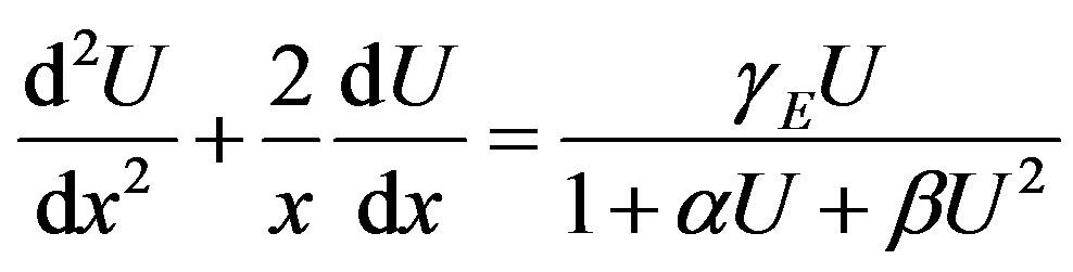
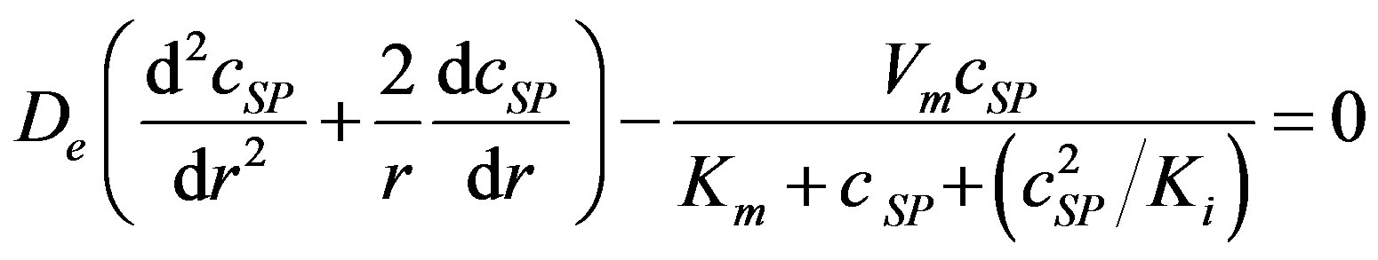 (5)
(5)
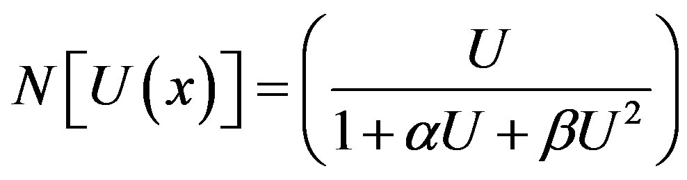
The system governs the substrate concentration  when there is no competitive inhibition in the reaction. The non-linear ODE (Eq.5) is made dimensionless by defining the following parameters:
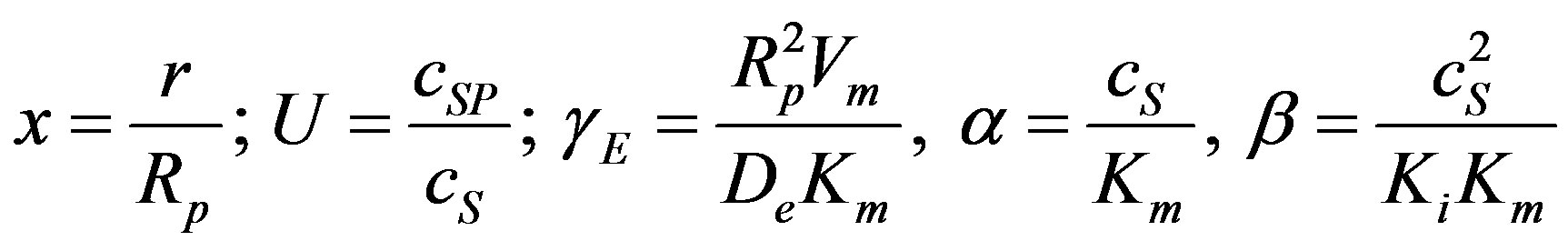 (6)
(6)
where  denote the reaction diffusion parameter, x is the dimensionless distance and
  is the dimensionless concentration. Here
  and
and  denotes the saturation parameters. The above Eq.5 reduces to the following dimensionless form
 (7)
(7)
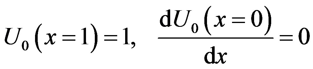
The corresponding boundary conditions are
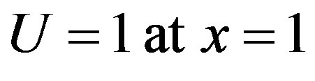 (8)
(8)
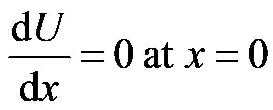 (9)
(9)
3. SOLUTION OF BOUNDARY VALUE PROBLEM USING ADOMIAN DECOMPOSITION METHOD
Adomian’s decomposition method has been successfully applied to linear and nonlinear problems. One of its advantages is that it provides a rapid convergent solution series [8]. However, the method applied to nonlinear Equations does not seem to be fast enough to be a efficient method to solve these kind of equations and one can find in the open literature some modifications proposed by several authors [9-13]. By applying the Adomian’s decomposition method, a new iterative method to compute nonlinear equations is developed and is presented in this work. The Adomian decomposition method is an extremely simple method [9-13] to solve non-linear differential equations. First iteration is enough. Furthermore, the obtained result is of high accuracy. Using this Adomian decomposition method (see appendix A and B),
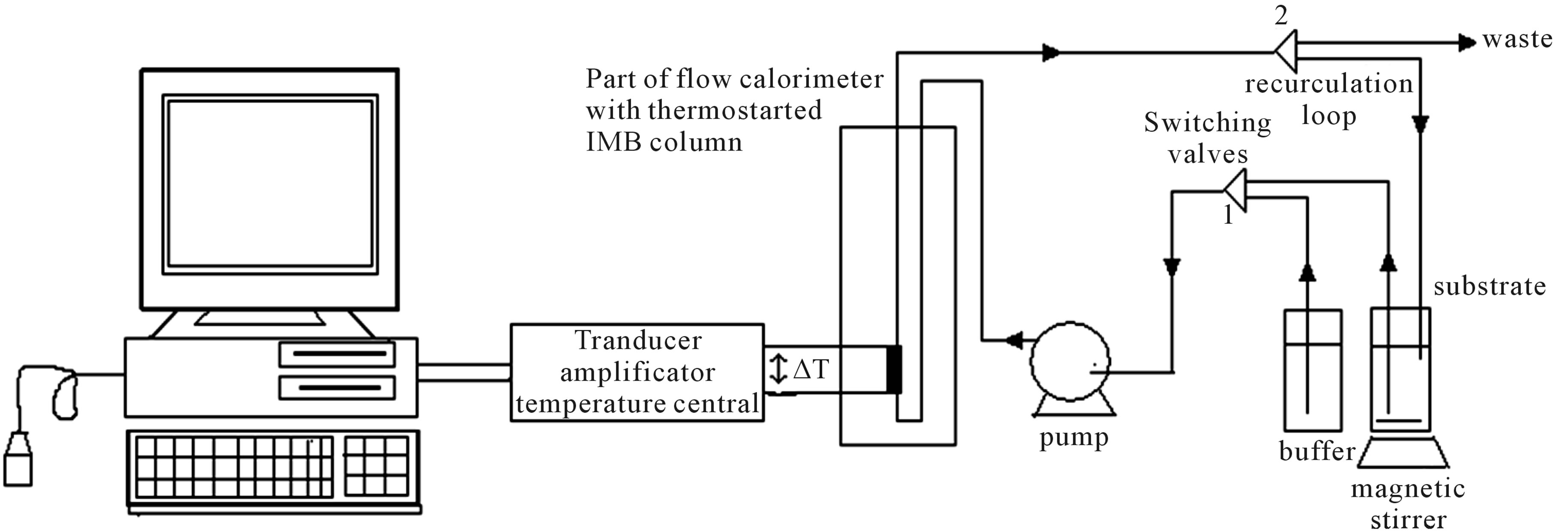
Figure 1. Experimental set-up of flow calorimetry.
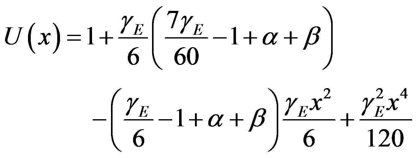
the solution of Eq.7 becomes:
 (10)
(10)
4. SOLUTION OF BOUNDARY VALUE PROBLEM USING HOMOTOPY ANALYSIS METHOD
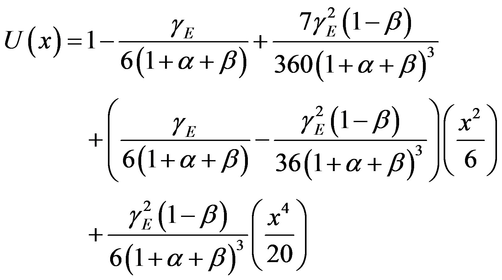
Perturbation methods are the most famous analytic techniques for nonlinear problems, which are widely applied in science and engineering. In 1992, the homotopy, a traditional concept in topology, was used by Liao [14] to propose an approximation technique for nonlinear problems, namely the homotopy analysis method (HAM). Using the concept of the homotopy, a nonlinear problem is transformed into a sequence of linear sub-problems that are easy to solve by means of the symbolic computation software. In 1997 Liao [14] further generalized the HAM by introducing an auxiliary nonzero parameter (called today the convergence-control parameter). Different from perturbation techniques, the HAM does not depend upon any small physical parameters, and besides provides great freedom to choose different base functions to approximate nonlinear problems. Especially, different from all other analytic approximation methods, the socalled convergence-control parameter of the HAM provides us a convenient way to ensure the convergence of series solution. Thus, the HAM overcomes the restrictions of the perturbation methods and therefore is more general. With these advantages and having the aid of high-performance computer and symbolic computation software, the HAM has been widely applied to solve many types of nonlinear differential Equations in science, engineering and finance [15]. Using this HAM (see Appendix C and D) we obtain, the concentration of substate as follows
 (11)
(11)
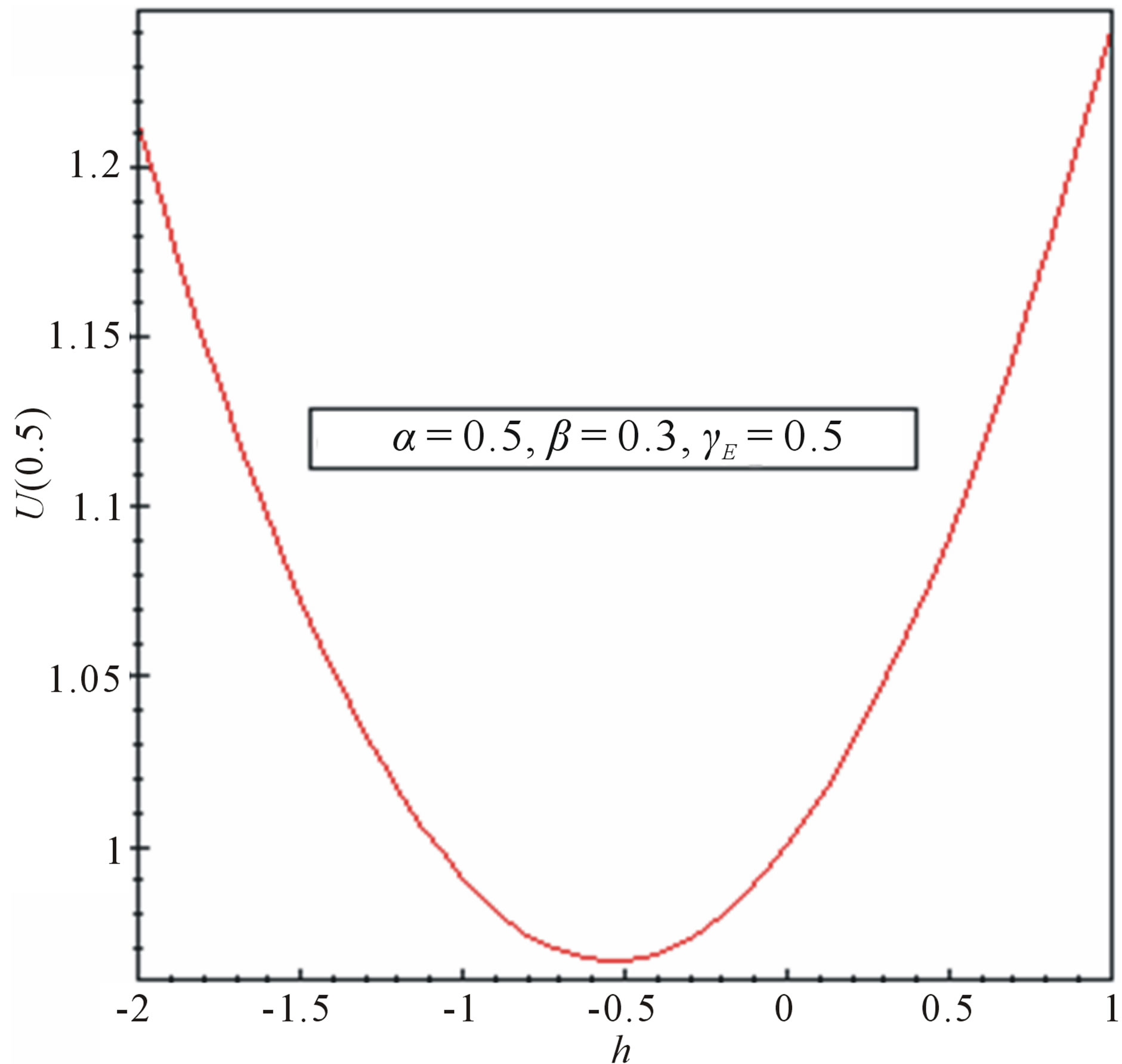
The analytical solution represented by Eq.11 contains the auxiliary parameter h, which gives the convergence region and rate of approximation for the homotopy analysis method. The analytical solution should converge. It should be noted that the auxiliary parameter h controls the convergence and accuracy of the solution series. In order to define region such that the solution series is independent of h, a multiple of h curves are plotted in Figure 2.
5. SOLUTION OF BOUNDARY VALUE PROBLEM USING HOMOTOPY PERTURBATION METHOD
The Homotopy perturbation method which doesn’t need small parameter is implemented for solving the
 (a)
(a)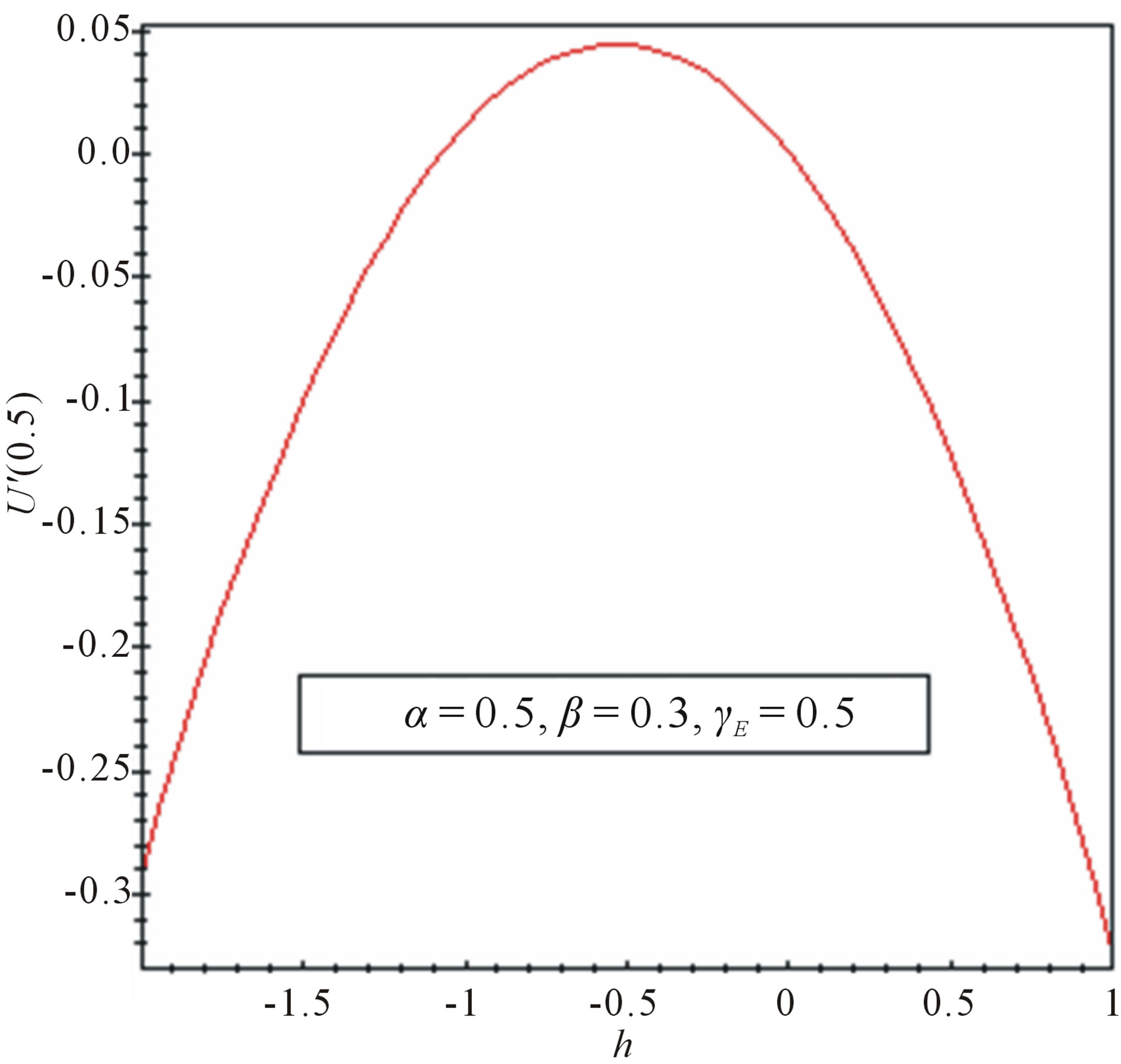 (b)
(b)
Figure 2. The h curves indicate the convergence region, for α = 0.5, β = 0.3 and γE = 0.5.
differential Equations and it is predicted that HPM can be founded widely applicable in engineering and in cases that don’t have exact solution this method can be used as semi-exact solution. Homotopy perturbation method yields a very rapid convergence and usually, one iteration leads to high accuracy of solution [17-25]. The Homotopy perturbation method is a high accuracy method. Using this method (see Appendix E and F) we obtain
 (12)
(12)
6. NUMERICAL SIMULATION
The non-linear differentials Eqs.7-9 are also solved by numerical methods. The function bvp4c in Matlab software which is a function of solving two-point boundary value problems (BVPs) for ordinary differential equations is used to solve this Equation. The Matlab program is also given in appendix G. Numerical values of the parameters used in Fedor Malik et al. [7] in this work is given in Table 1. Its numerical solution is compared with Adomian decomposition method, Homotopy analysis and perturbation method in Table 2-5 and it gives satisfactory result when α ≤ 1 and β ≤ 1.
7. RESULTS AND DISCUSSION
The primary result of this work is the first approximate and simple expression of concentrations of substrate (Eqs.10 (ADM), 11 (HAM) and 12 (HPM)). Figures 3-6 show the analytical expression of concentration of substrate  for various values of dimensionless reaction diffusion parameter
  and saturation parameters
 . From these Figures 3-6, it is inferred that the value of the concentration of substrate
  increases when dimensionless reaction diffusion parameter
  decreases. Also in these Figures 3 to 6, it is known that the value of the concentration of substrate increases gradually and attains the maximum at the boundary
 .
.
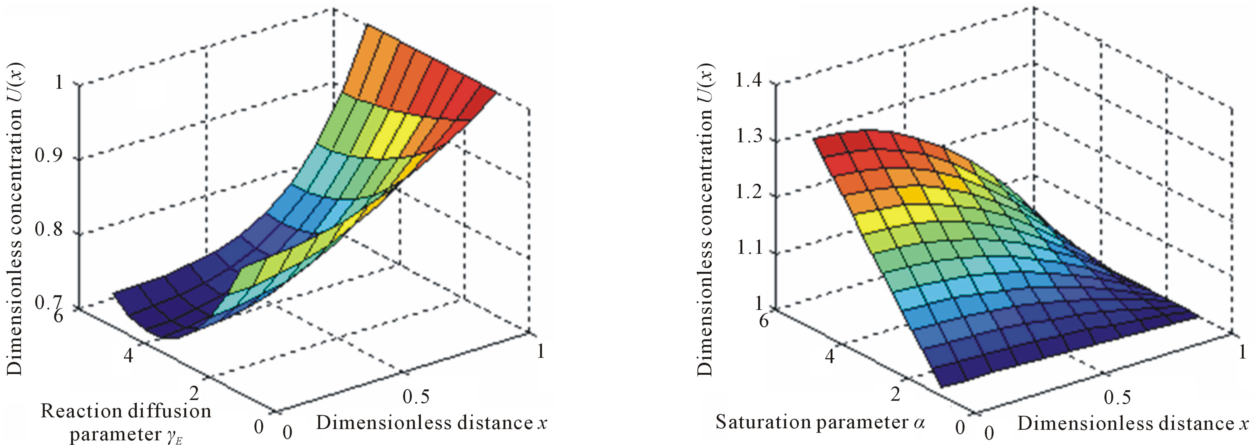
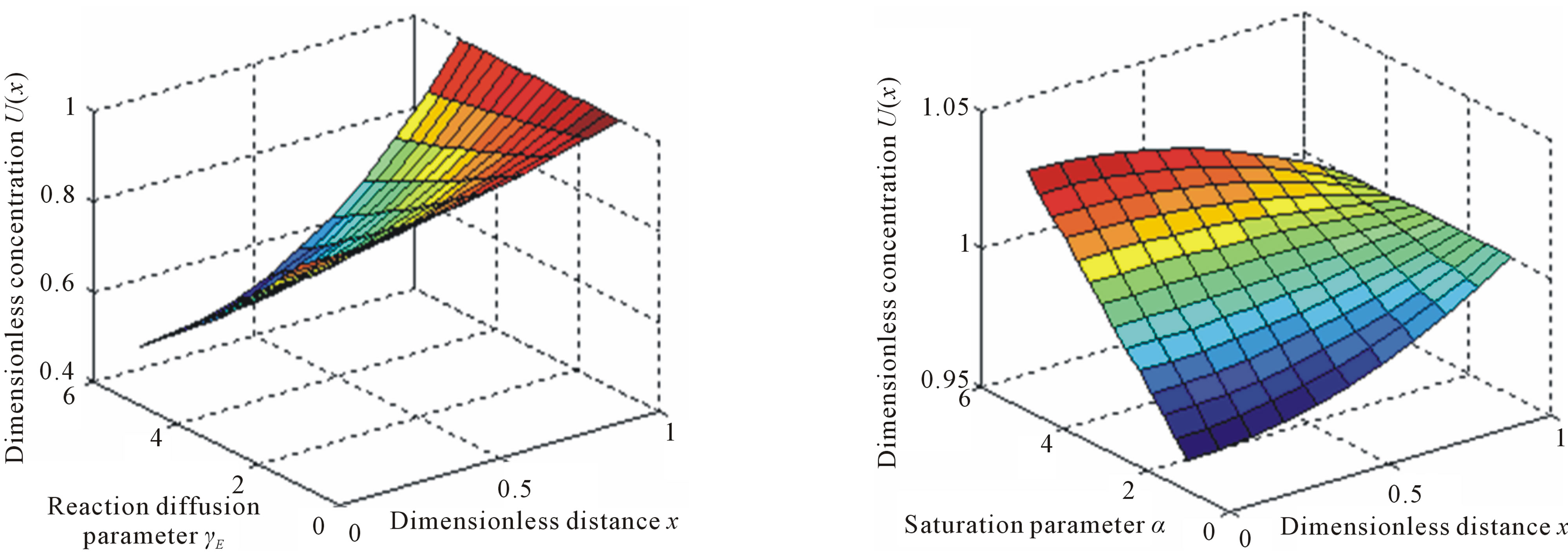
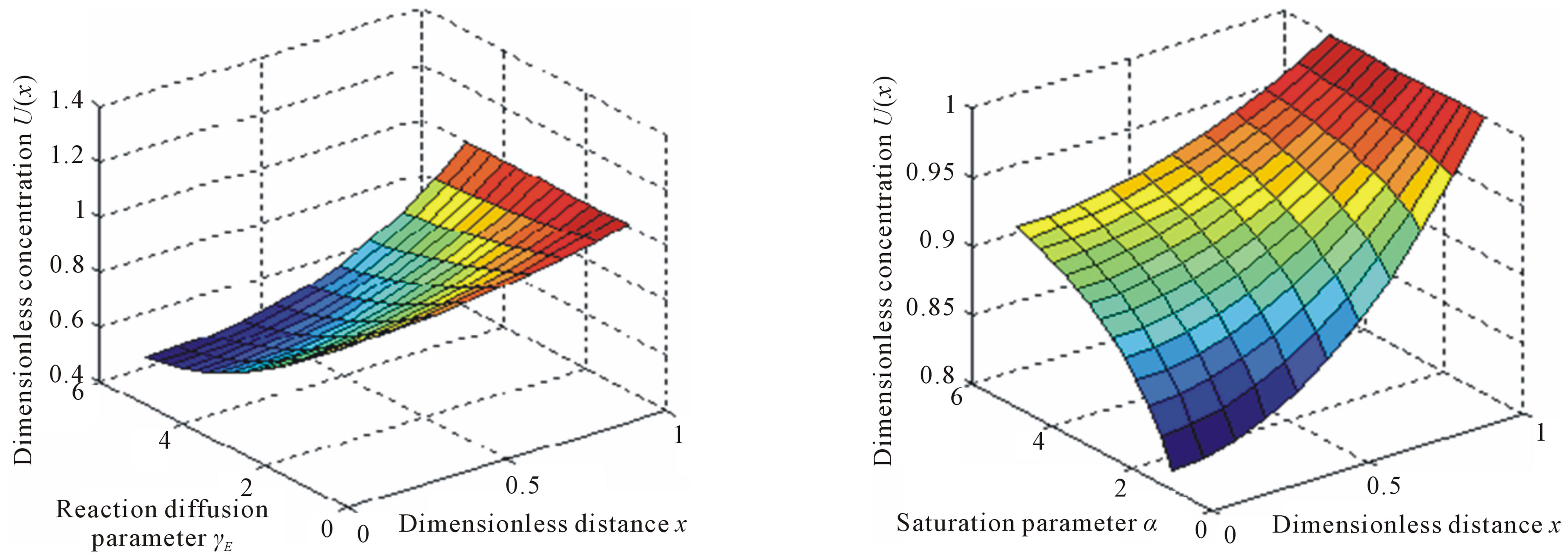
The normalized numerical simulation of three dimensional substrate concentration  is shown in Figures 7-9. The time independent concentration
  is represented in Figures 7-9 for fixed value of
 . Concentration
  is slowly decreasing when
  is increasing. Then the concentration of
  when
when  and also for all values of
 ,
,  and
and . In these figure, it should be noted that the value of the concentration of substrate decreases for all values of
 . From this figures, it is apparent that the value of the concentration of substrate increases for various values of
  increases.
8. CONCLUSION
A non-linear ordinary differential equation in the investigation of kinetics of immobilized liver esterase by flow calorimetry has been solved using Adomian decomposition method, Homotopy analysis and perturbation method. The simple approximate expression of concentration of substrate for all values of parameters  and
and  are reported. These methods can be easily extended to find the solution of all other non-linear reaction diffusion equations for immobilized enzymes with reversible Michaelis-Menten kinetics for various complex boundary conditions. These analytical results are useful for design and optimization of immobilized liver esterase by flow calorimetry.
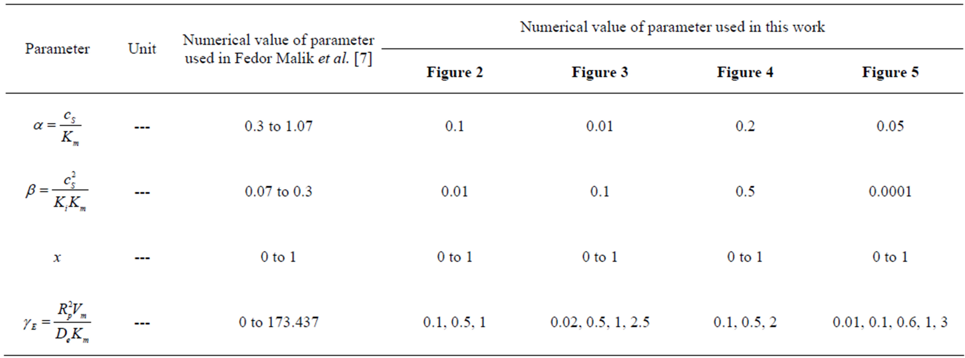
Table 1. Numerical values of the parameters used in this work. The fixed values of the dimension parameters are cS = 3.24, 5.932 mmold∙m−3, De = 9.4 × 10⁻⁹ dm2∙s−1, Ki = 25, 17 mmold∙m−3, Km = 9, 6.4 mmold∙m−3, Vm = 13.7, 11.1 mK and Rp = 0.001. These are dimensional parameters used in Fedor Malik et al. [7].
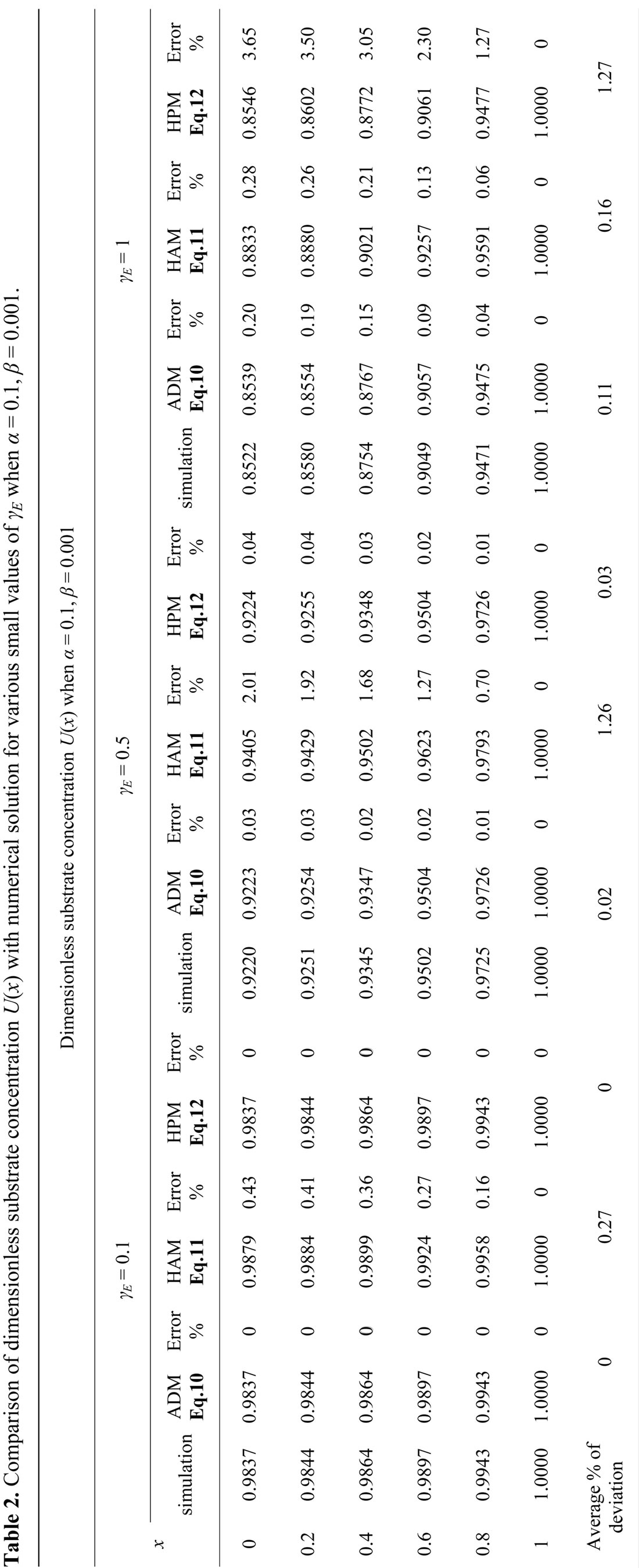
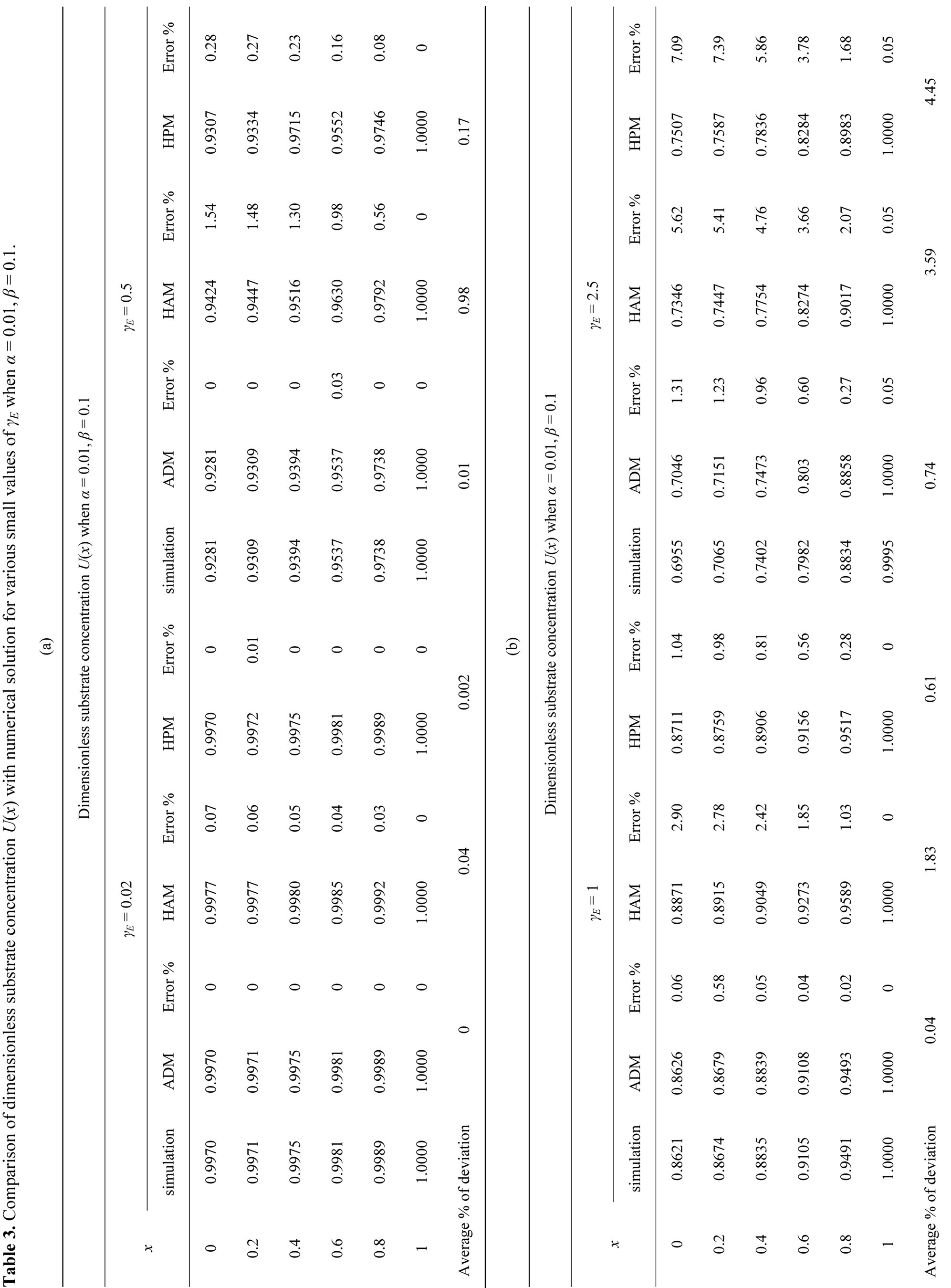
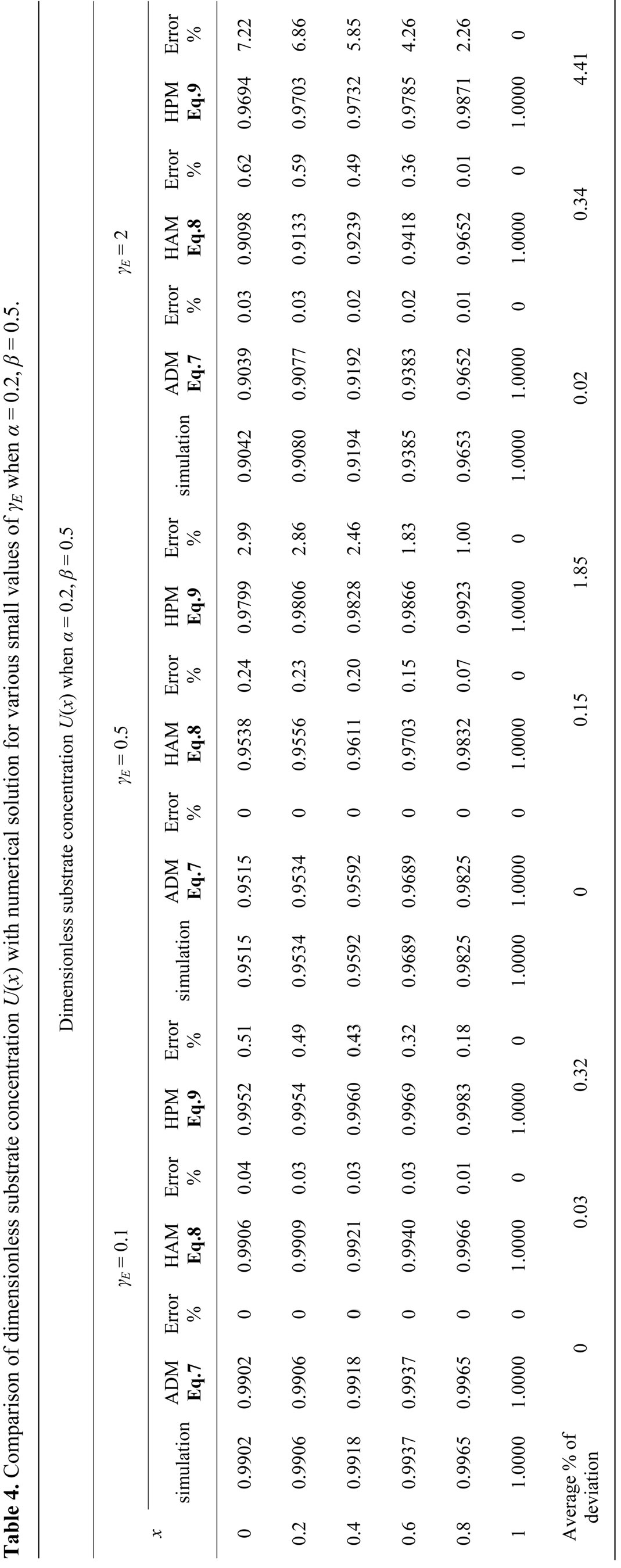
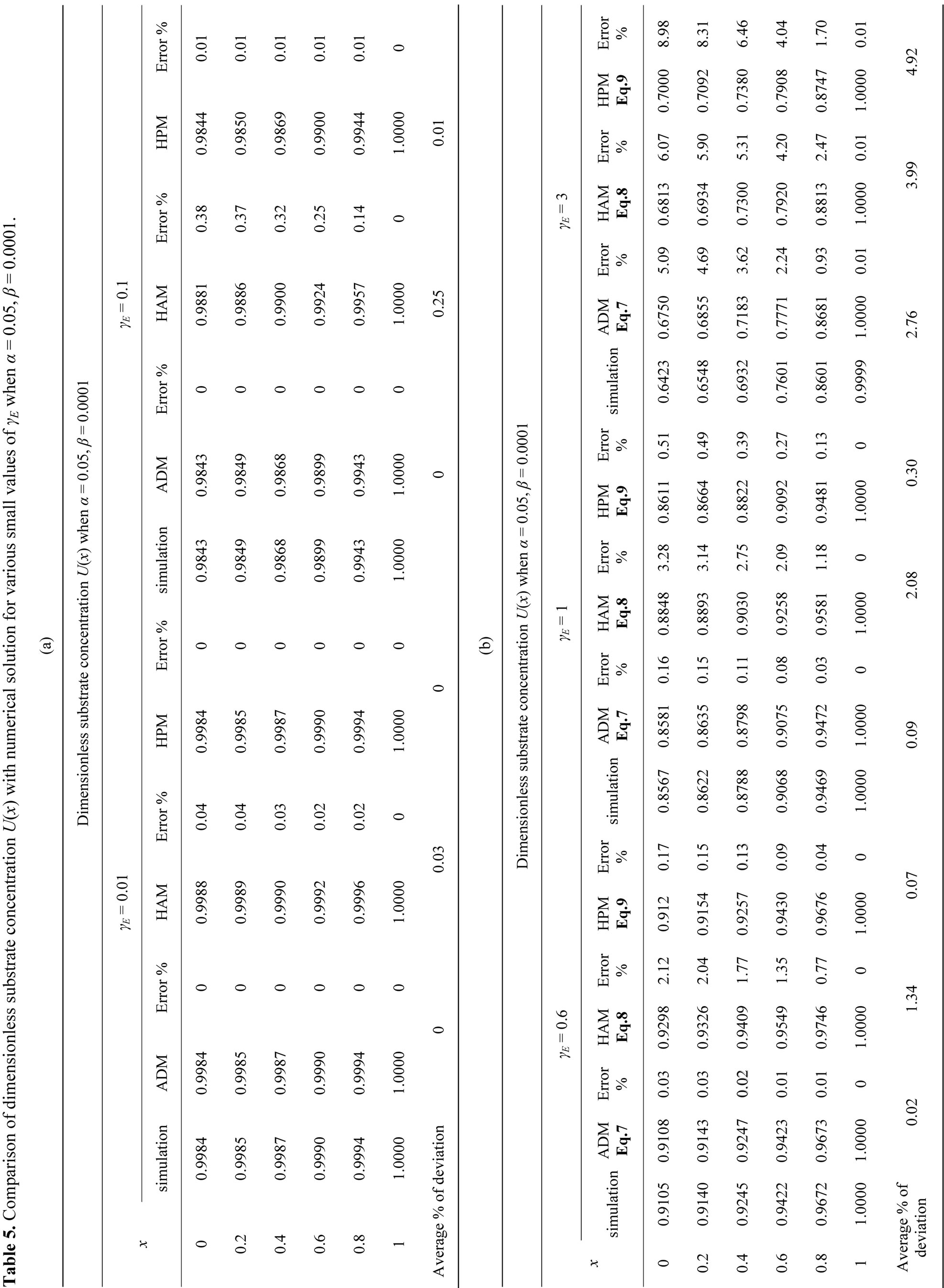
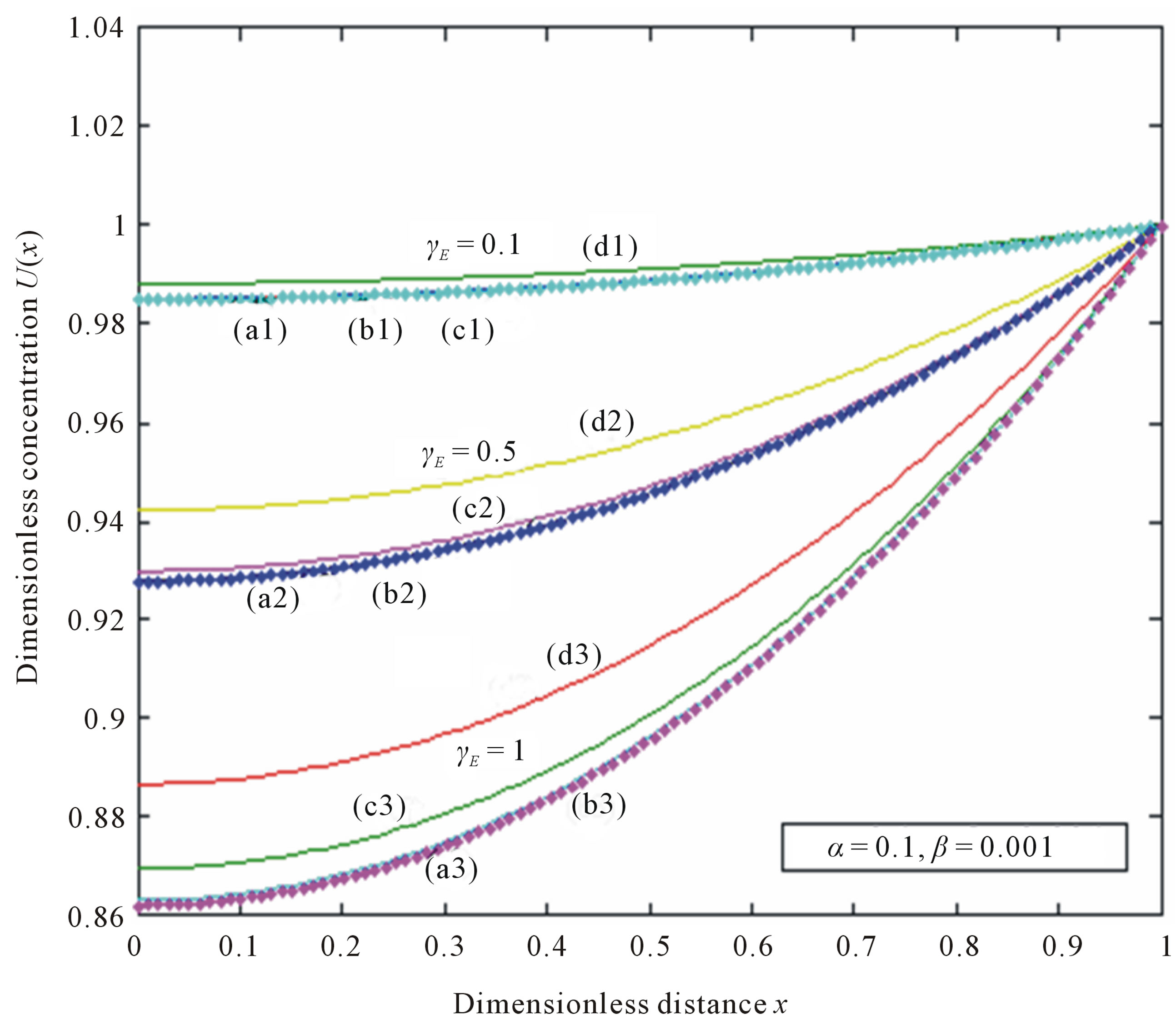
Figure 3. Dimensionless concentration U(x) versus dimensionless distance x when α = 0.1, β = 0.001. The curves a1, a2, a3 (ADM), b1, b2, b3 (simulation), c1, c2, c3 (HPM), d1, d2, d3 (HAM) are plotted when γE = 0.1, 0.5, 1. Symbols (---) Eqs. 10-12 and (…) numerical simulation.
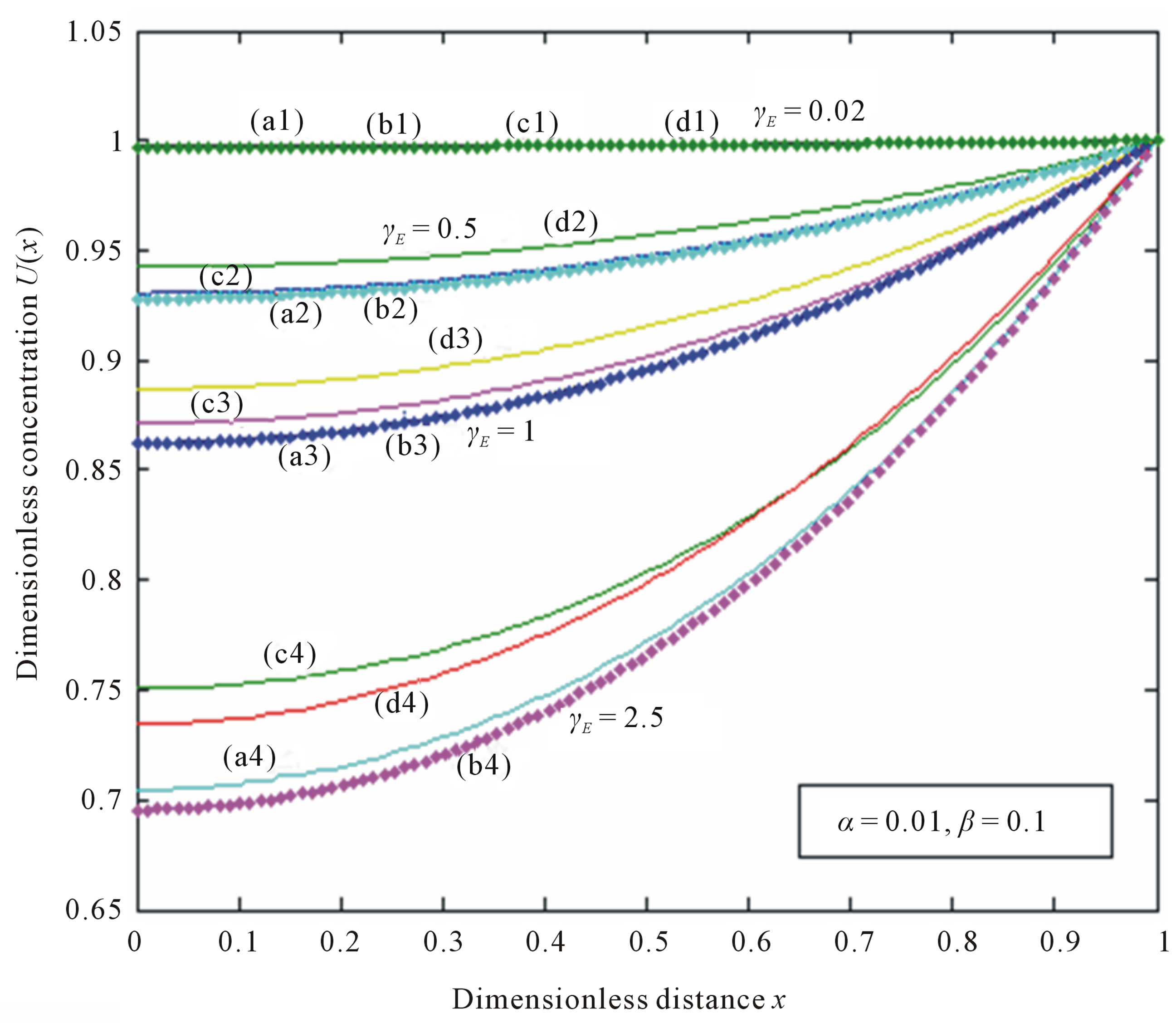
Figure 4. Dimensionless concentration U(x) versus dimensionless distance x when α = 0.01, β = 0.1. The curves a1, a2, a3, a4 (ADM), b1, b2, b3, b4 (simulation), c1, c2, c3, c4 (HAM), d1, d2, d3, d4 (HPM) are plotted when γE = 0.02, 0.5, 1, 2.5. Symbols (---) Eqs.10-12 and (…) numerical simulation.
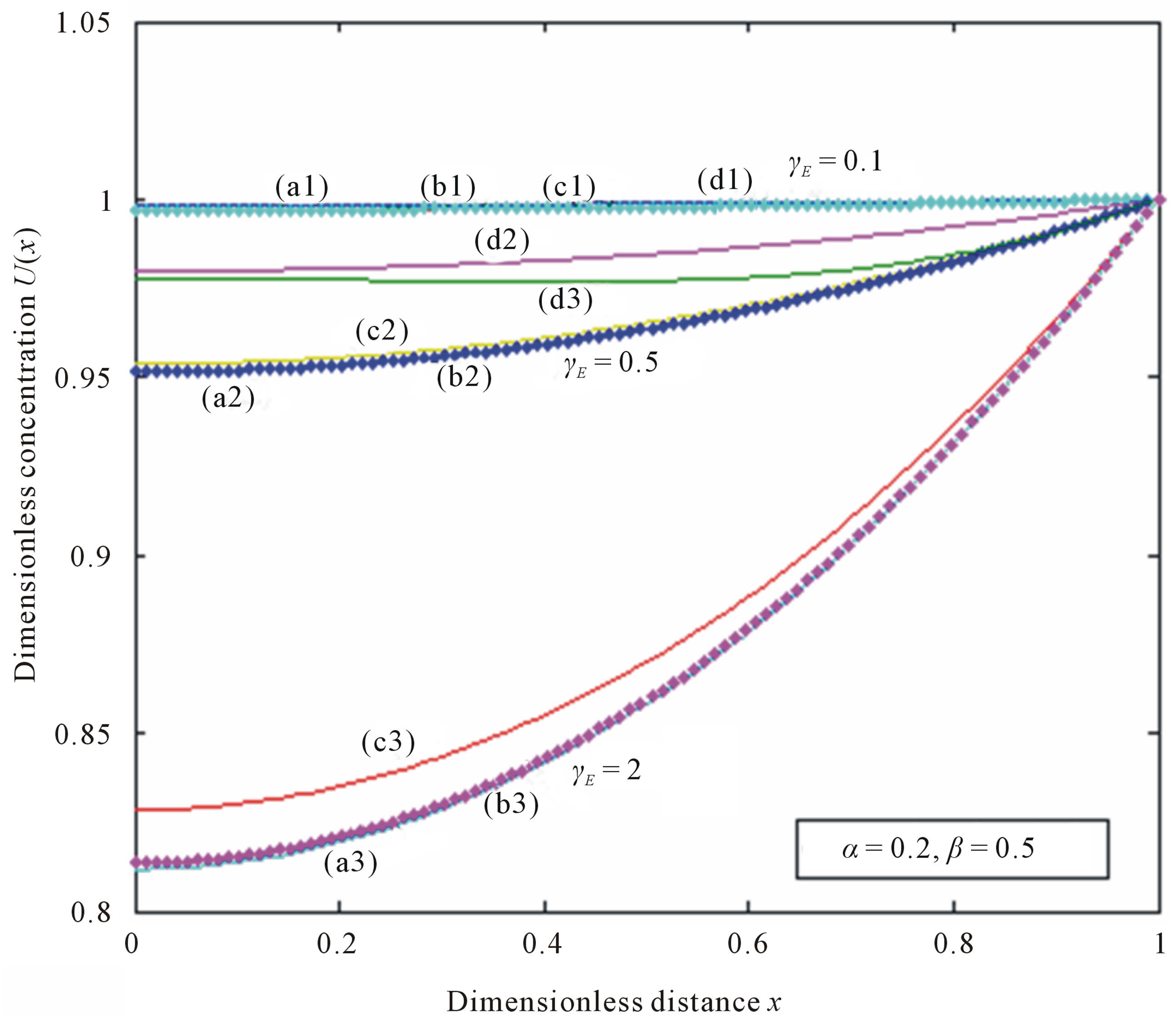
Figure 5. Dimensionless concentration U(x) versus dimensionless distance x when α = 0.2, β = 0.5. The curves a1, a2, a3 (ADM), b1, b2, b3 (simulation), c1, c2, c3 (HAM), d1, d2, d3 (HPM) are plotted when γE = 0.1, 0.5, 2. Symbols (---) Eqs.10-12 and (…) numerical simulation.
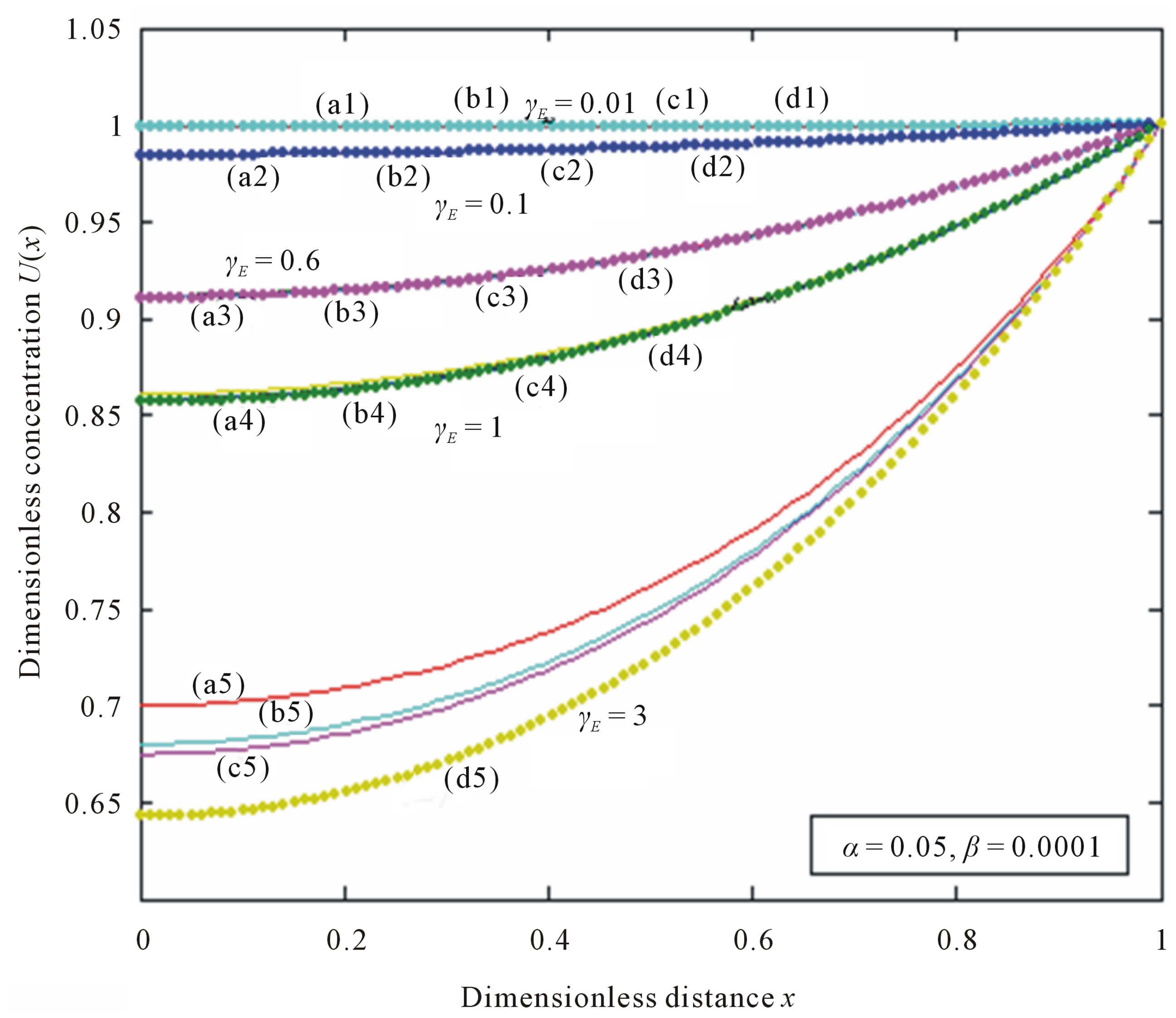
Figure 6. Dimensionless concentration U(x) versus dimensionless distance x when α = 0.05, β = 0.0001. The curves a1, a2, a3, a4, a5 (HPM), b1, b2, b3, b4, b5 (HAM), c1, c2, c3, c4, c5 (ADM), d1, d2, d3, d4, d5 (simulation) are plotted when γE = 0.01, 0.1, 0.6, 1, 3. Symbols (---) Eqs.10-12 and (…) numerical simulation.
 (a) (b)
Figure 7. The normalized three dimensionless steady-state concentration profiles U(x) calculated using Eq.10. The plot was constructed for the values of α = 0.1 and β = 0.001, β = 0.001 and γE = 0.1.
 (a) (b)
Figure 8. The normalized three dimensionless steady-state concentration profiles U(x) calculated using Eq.11. The plot was constructed for the values of α = 0.1 and β = 0.001, β = 0.001 and γE = 0.1.
 (a) (b)
Figure 9. The normalized three dimensionless steady-state concentration profiles U(x) calculated using Eq.12. The plot was constructed for the values of α = 0.1 and β = 0.001, β = 0.001 and γE = 0.1.
9. ACKNOWLEDGEMENTS
This work was supported by the UGC and CSIR, Government of India. The authors are grateful to Dr. R. Murali, the Principal, the Madura College, Madurai, and the Secretary, the Madura College Board, Madurai, for their encouragement. We thank the reviewers for their valuable coments to improve the quality of the manuscript.
REFERENCES
- Monk, P. and Wadso, I. (1968) A flow micro reaction. Acta Chemica Scandinavica, 22, 1842-1852. doi:10.3891/acta.chem.scand.22-1842
- Burch, J. (1954) The purification and properties of horse liver esterase. Biochemistry, 58, 415-426.
- Stoops, J.K., Horgan, D.J., Runnegar, M.T.C., Jersey, J., de webb, E.C. and Zerner, B. (1969) Carboxylesterases (EC 3.1.1). Kinetic Studies on Carboxylesterases Biochemistry, 8, 2026-33.
- Adler, A.J. and Kistiakowasky, G.B. (1962) Kinetics of pig liver esterase catalysis. Journal of the American Chemical Society, 84, 695-703. doi:10.1021/ja00864a001
- Stefuca, V., Gemenier, P. and Scheper, V., Eds. (1999) Advances in biochemical engineering biotechnology. Springer, Berlin, 71.
- Stefuca, V., Vikartovska-Welwardova, V. and Gemenier, P. (1999) Flow microcalorimeter auto-calibration for the analysis of immobilized enzyme kinetics. Analytica Chimica Acta, 355, 63. doi:10.1016/S0003-2670(97)81612-1
- Stefuca, V., Cipakova, I. and Gemeine, P. (2001) Investigation of immobilized glucoamy lase kinetics by flow calorimetry. Thermochimica Acta, 378, 79-85. doi:10.1016/S0040-6031(01)00589-5
- Malik, F., Stefuca, V. and Bales, V. (2004) Investigation of kinetics of immobilized liver esterase by flow calorimetry. Journal of Molecular Catalysis B: Enzymatic, 29, 81-87. doi:10.1016/S0040-6031(01)00589-5
- Jaradat, O.K. (2008) Adomian decomposition method for solving abelian differential equations. Journal of Applied Sciences, 8, 1962-1966. doi:10.1016/S0040-6031(01)00589-5
- Majid Wazwaz, A. and Gorguis, A. (2004) The decomposition method applied to systems of partial differential equations. Applied Mathematics and Computation, 149, 807-814.
- Makinde, O.D. (2007) Adomian decomposition approach to a SIR epidemic model with constant vaccination strategy. Applied Mathematics and Computation, 184, 842- 848. doi:10.1016/j.amc.2006.06.074
- Siddiqui, A.M., Hameed, M., Siddiqui, B.M. and Ghori, Q.K. (2010) Use of Adomian decomposition method in the study of parallel plate flow of a third grade fluid. Communications in Nonlinear Science and Numerical Simulation, 15, 2388-2399. doi:10.1016/j.cnsns.2009.05.073
- Mohamed, M.A. (2010) Comparison differential transformation technique with Adomian decomposition method for dispersive long-wave equations in (2+1)-dimensions. Applied Mathematics, 5, 148-166.
- Liao, S.J. (1992) The proposed homotopy analysis technique for the solution of nonlinear problems. Ph.D. Thesis, Shanghai Jiao Tong University, Shanghai.
- Liao, S.J. (2003) Beyond perturbation: Introduction to the homotopy analysis method. CRC Press, Boca Raton. doi:10.1201/9780203491164
- Awaadeh, F., Jaradat, H.M. and Alsyyed, O. (2009) Analytical solution for nonlinear gas dynamic equation by homotopy analysis method. Chaos, Solitons & Fractals, 42, 1422-1427.
- Jafari, H., Chun, C. and Saeidy, S. (2009) Analytical solution for nonlinear gas dynamic equation by homotopy analysis method. Applied Mathematics, 4, 149-154.
- Sohouli, A.R., Famouri, M., Kimiaeifar, A. and Domairry, G. (2010) Application of homotopy analysis method for natural convection of Darcian fluid about a vertical full cone embedded in pours media prescribed surface heat flux. Communications in Nonlinear Science and Numerical Simulation, 15, 1691-1999. doi:10.1016/j.cnsns.2009.07.015
- Domarriy, G. and Fazeli, M. (2009) Homotopy analysis method to determine the fin efficiency of convective straight fins with temperature-dependent thermal conductivity. Communications in Nonlinear Science and Numerical Simulation, 14, 489-499. doi:10.1016/j.cnsns.2007.09.007
- Liao, S.J. (2004) On the homotopy analysis method for nonlinear problems. Applied Mathematics and Computation, 147, 499-513. doi:10.1016/S0096-3003(02)00790-7
- Domairry, G. and Barring, H. (2008) An approximation of the analytic solution of some nonlinear heat transfer equations: A survey by using homotopy analysis method. Advanced Studies in Theoretical Physics, 2, 507-518.
- He, J.H. (2000) A coupling method of homotopy technique and a perturbation technique for non-linear problems. International Journal of Non-Linear Mechanics, 35, 37-43. doi:10.1016/S0020-7462(98)00085-7
- Ganji, D.D., Amini, M. and Kolahdooz, A. (2008) Analytical investigation of hyperbolic equations via He’s methods. American Journal of Engineering and Applied Sciences, 1, 399-407. doi:10.3844/ajeassp.2008.399.407
- Ariel, P.D. (2010) Homotopy perumbation method and natural convention flow of a third grade fluid through a circular tubenon. Nonlinear Science Letters A, 1, 43-52.
- Fereidoon, A., Rostamiyan, Y., Davoudabadi, M.R., Farahani, S.D. and Ganji, D.D. (2010) Analytic approach to investigation of distributions of stresses and radial displacement at the thick-wall cylinder under the internal and external pressures. Middle-East Journal of Scientific Research, 5, 321-328.
APPENDIX A
Basic Concept of the Adomian Decomposition Method (ADM)
Adomian decomposition method [9-13] depends on the non-linear differential equation
 (A.1)
(A.1)
into the two components
 (A.2)
(A.2)
where L and N are the linear and non-linear parts of F respectively. The operator L is assumed to be an invertible operator. Solving for  leads to
 (A.3)
(A.3)
Applying the inverse operator L on both sides of Eq. A.3 yields
 (A.4)
(A.4)
where  is the constant of integration which satisfies the condition
  Now assuming that the solution
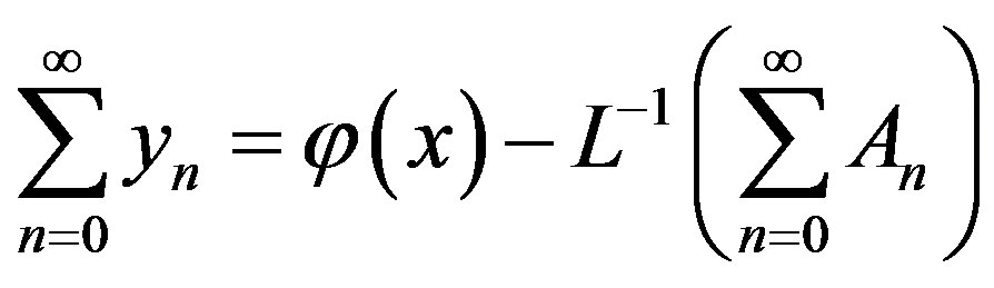
  can be represented as infinite series of the form
 (A.5)
(A.5)
Furthermore, suppose that the non-linear term  can be written as infinite series in terms of the Adomian polynomials
  of the form
 (A.6)
(A.6)
where the Adomian polynomials  of
of  are evaluated using the formula:
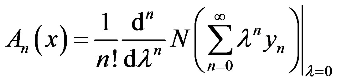 (A.7)
(A.7)
Then substituting Eqs.A.5 and A.6 in Eq.A.4 gives
 (A.8)
(A.8)
Then equating the terms in the linear system of Eq. A.8 gives the recurrent relation
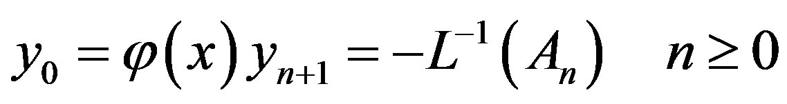 (A.9)
(A.9)
However, in practice all the terms of series in Eq.A.7 cannot be determined, and the solution is approximated by the truncated series . This method has been proven to be very efficient in solving various types of non-linear boundary and initial value problems.
APPENDIX B
Analytical Solutions of Concentrations of Substrate Using ADM
In this appendix, we derive the general solution of nonlinear Eq.7 by using Adomian decomposition method. We write the Eq.7 in the operator form,
 (B.1)
(B.1)
where . Applying the inverse operator
  on both sides of Eq.B.1 yields
 (B.2)
(B.2)
where A and B are the constants of integration. We let,
 (B.3)
(B.3)
 (B.4)
(B.4)
where
 (B.5)
(B.5)
In view of Eqs.B.3-B.5, Eq.B.2 gives
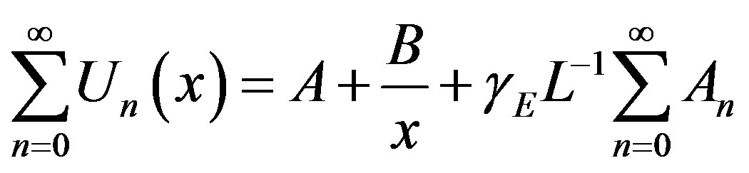 (B.6)
(B.6)
We identify the zeroth component as
 (B.7)
(B.7)
and the remaining components as the recurrence relation
 (B.8)
(B.8)
where An are the Adomian polynomials of . We can find the first few An as follows:
 (B.9)
(B.9)
 (B.10)
The remaining polynomials can be generated easily, and so,
 (B.11)
 (B.12)
 (B.13)
Adding (B.11) to (B.13) we get Eq.11 in the text.
APPENDIX C
Basic Concept of Homotopy Analysis Method
Consider the following differential equation [15]:
 (C.1)
(C.1)
where Ν is a nonlinear operator, t denotes an independent variable; u(t) is an unknown function. For simplicity, we ignore all boundary or initial conditions, which can be treated in the similar way. By means of generalizing the conventional homotopy method, Liao constructed the so-called zero-order deformation equation
 (C.2)
(C.2)
where  is the embedding parameter,
  is a nonzero auxiliary parameter,
  is an auxiliary function, L is an auxiliary linear operator,
  is an initial guess of
 ,
,  is an unknown function. It is an important, that one has great freedom to choose auxiliary unknowns in HAM. Obviously, when p = 0 and p = 1, it holds:
 (C.3)
(C.3)
respectively. Thus, as p increases from 0 to 1, the solution  varies from the initial guess
  to the solution
  Expanding
  in Taylor series with respect to p, we have
 (C.4)
(C.4)
where
 (C.5)
(C.5)
If the auxiliary linear operator, the initial guess, the auxiliary parameter h, and the auxiliary function are so properly chosen, the series (C.4) converges at p = 1 then we have:
 . (C.6)
Define the vector
 (C.7)
(C.7)
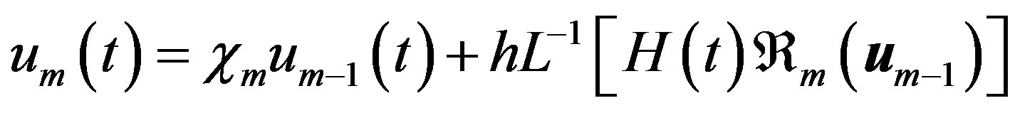
Differentiating Eq.C.2 for m times with respect to the embedding parameter p, and then setting p = 0 and finally dividing them by m! we will have the so-called  -order deformation Equation as:
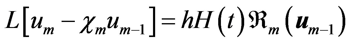 (C.8)
(C.8)
where
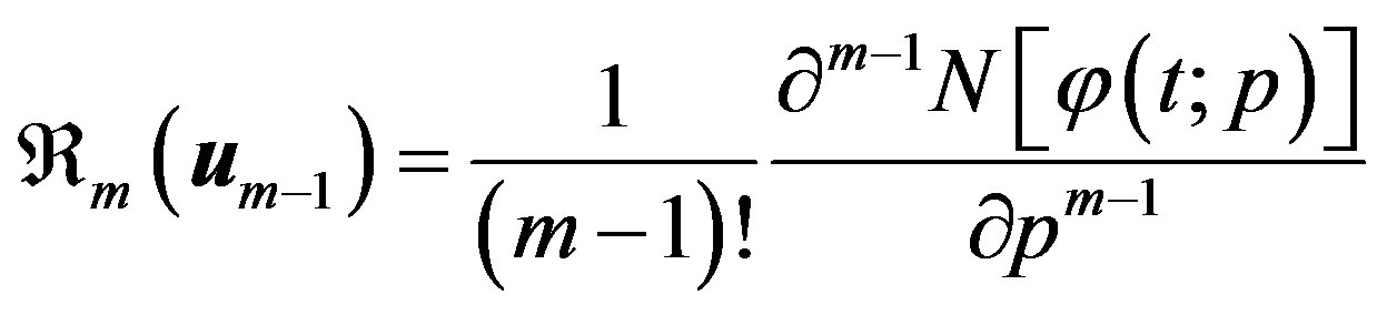 (C.9)
(C.9)
And
 (C.10)
Applying  on both side of Eq.A8, we get
 (C.11)
In this way, it is easily to obtain  for
for  at
at  order, we have
 (C.12)
when , we get an accurate approximation of the original Eq.C.1. For the convergence of the above method we refer the reader to Liao [15]. If Eq.C.1 admits unique solution, then this method will produce the unique solution. If Eq.C.1 does not possess unique solution, the HAM will give a solution among many other (possible) solutions.
APPENDIX D
Approximate Analytical Solutions of the System of Eqs.7-9 Using HAM
In this appendix, we indicate how Eq.11 in this paper is derived. The Homotopy analysis method was constructed to determine the solution of Eqs.7-9.
 (D.1)
(D.1)
In order to solve Eq.D.1 by means of the HAM, we first construct the zeroth-order deformation Equation by taking ,
,
 (D.2)
(D.2)
The approximate solutions of Eq.D.2 are as follows
 (D.3)
(D.3)
Substituting the series (D.3) in Eq.D.2 and equating the like powers of p we get
 (D.4)
(D.4)
 (D.5)
(D.5)
 (D.6)
(D.6)
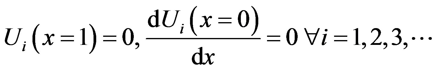
The boundary conditions becomes
 (D.7)
(D.7)
and
 (D.8)
(D.8)
Now applying the boundary conditions Eq.D.7 in Eq. D.4 we get
 (D.9)
(D.9)
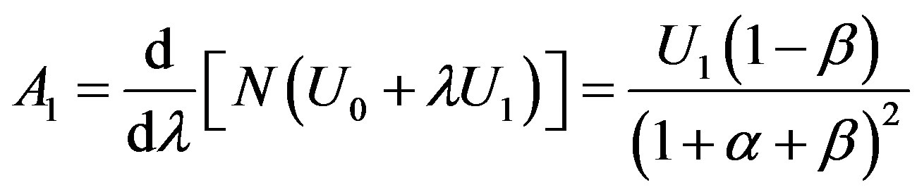
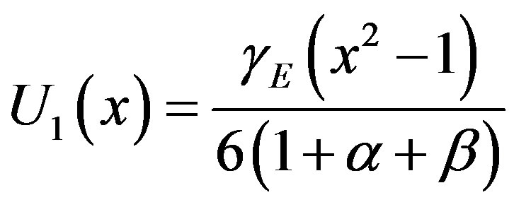
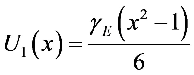
Substituting the values of  in Eq.D.5 and solving the Equation using the boundary conditions Eq.D.8 we obtain the following result:
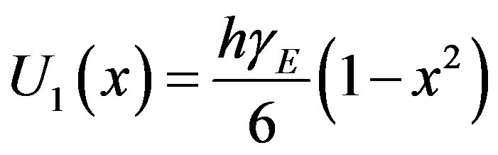 (D.10)
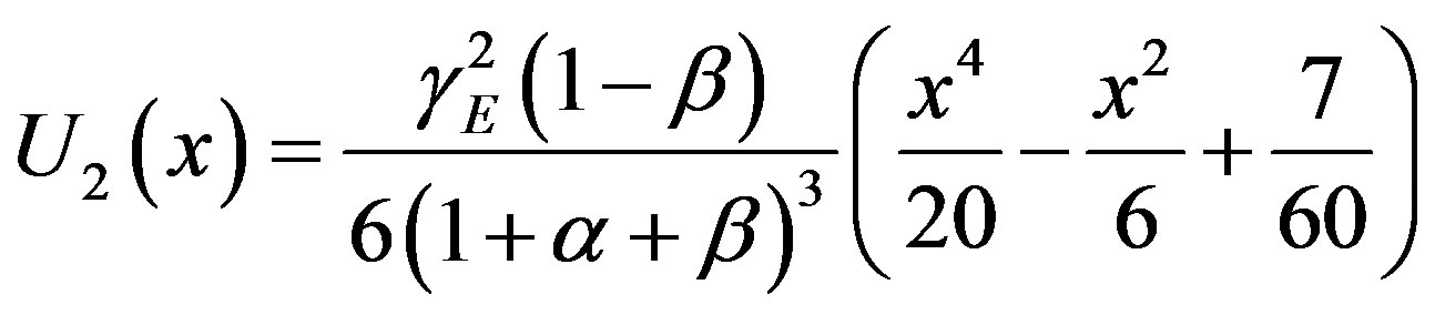
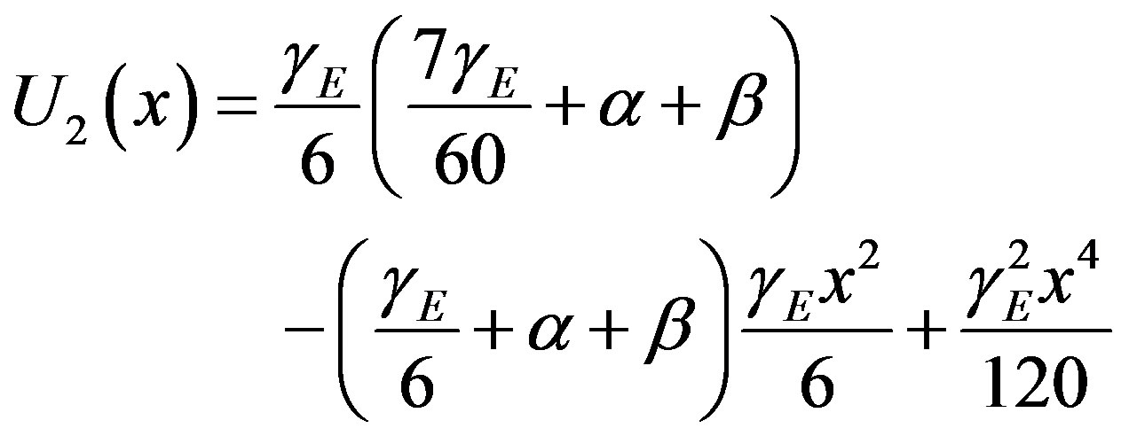
Substituting the values of U0 and U1 in Eq.D.6 and solving the Equation using the boundary conditions Eq. D.8 we obtain the following result:
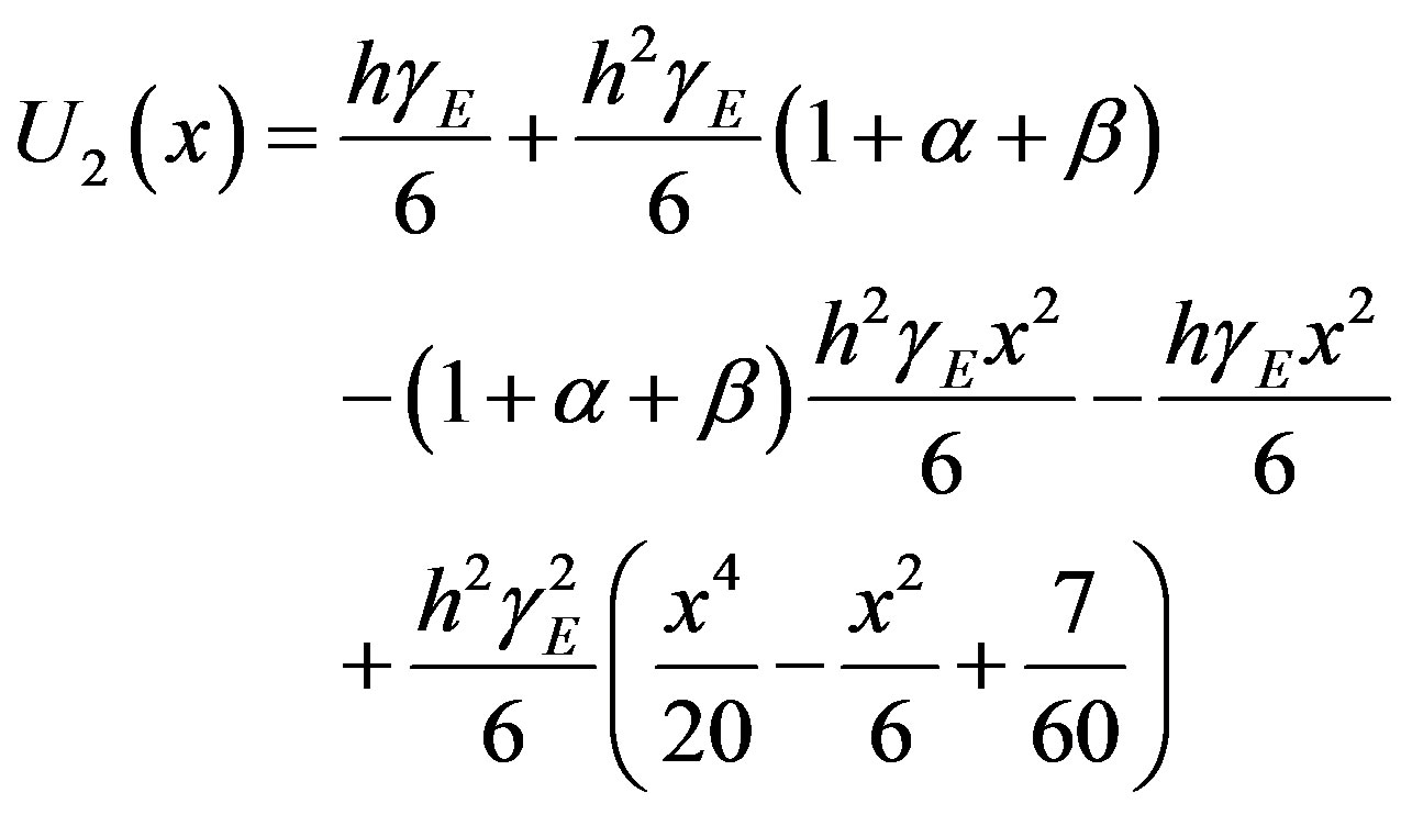 (D.11)
To find few iteration we get, the solution of  to reach the better approximation. Adding (D.9), (D.10) and (D.11), we get Eq.11 in the text.
APPENDIX E
Basic Concept of the Homotopy Perturbation Method (HPM)
We outline the basic idea of Homotopy perturbation method. This method has eliminated the limitations of the traditional perturbation methods. On the other hand it can take full advantage of the traditional perturbation techniques, so there has been a considerable deal of research in applying homotopy technique for solving various strongly non-linear equations. To explain this method, let us consider the following function
 (E.1)
(E.1)
with the boundary conditions of
 (E.2)
(E.2)
where ,
, ,
, and
and  denote a general differential operator, a boundary operator, a known analytical function and the boundary of the domain
 , respectively. Generally speaking, the operator A can be divided into a linear part L and a non-linear part N. Eq.2.1 can therefore be written as
 (E.3)
(E.3)
By the homotopy perturbation technique, we construct a homotopy  which satisfies
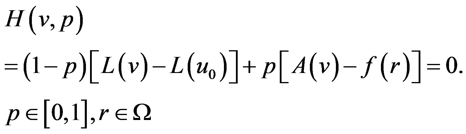 (E.4)
(E.4)
or
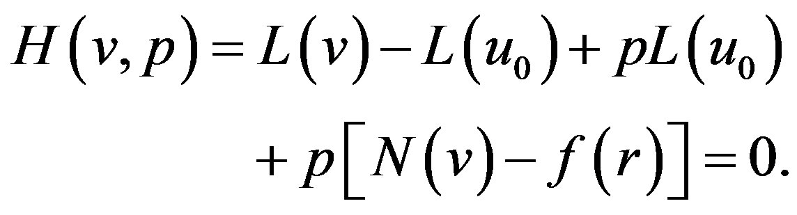 (E.5)
(E.5)
where  is an embedding parameter, and
  is an initial approximation of Eq.E.1, which satisfies the boundary conditions. Obviously from Eqs.E.4 and E.5, we will have
 (E.6)
(E.6)
 (E.7)
(E.7)
when p = 0 Eq.E.4 or E.5 becomes a linear Equation; when p = 1 it becomes a non-linear Equation. So the changing process of p from zero to unity is just that of  to
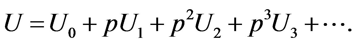
to . We can first use the embedding parameter p as a “small parameter”, and assume that the solutions of Eqs.E.4 and E.5 can be written as a power series in p
 (E.8)
(E.8)
Setting p = 1, results in the approximate solution of Eq.E.1:
 (E.9)
(E.9)
The combination of the perturbation method and the Homotopy method is called the Homotopy perturbation method.
APPENDIX F
Approximate Analytical Solutions of the system of Eqs.7-9 Using HPM
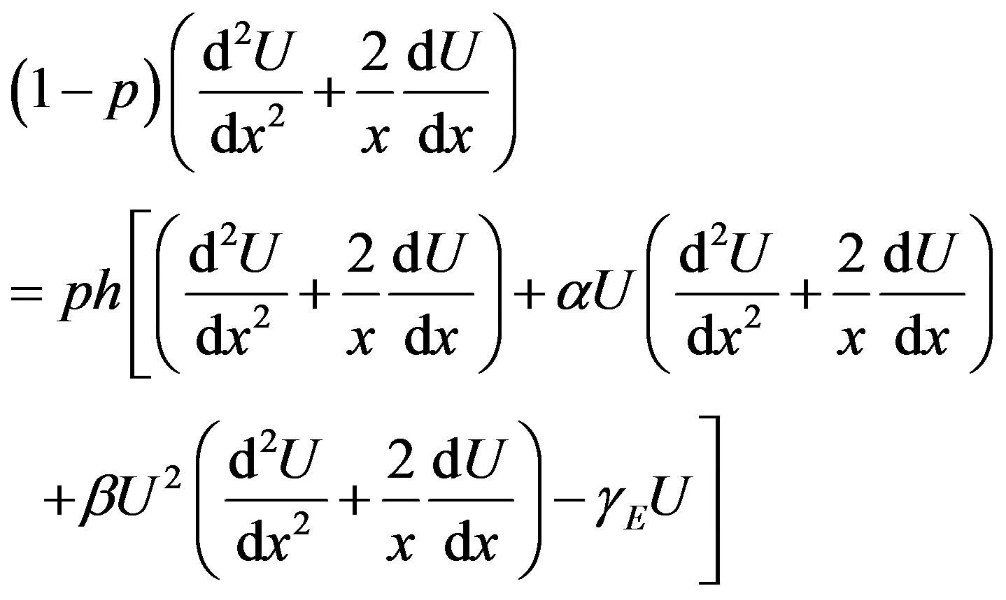
Solution of the Eqs.7-9 using Homotopy perturbation method. In this appendix, we indicate how Eq.12 in this paper is derived. Furthermore, a Homotopy was constructed to determine the solution of Eqs.7.
 (F.1)
(F.1)
The approximate solutions of Eq.F.1 is
 (F.2)
(F.2)
Substituting Eq.F.2 into Eq.F.1, and comparing the coefficients of like powers of p
 (F.3)
(F.3)
 (F.4)
(F.4)
 (F.5)
(F.5)
The boundary conditions are
 (F.6)
(F.6)
and
 (F.7)
(F.7)
Solving the Eqs.F.3 to F.5 and using the boundary conditions (F.6) and (F.7), we can find the following results
 (F.8)
(F.8)
 (F.9)
(F.9)
 (F.10)
According to the HPM, we can conclude that
 (F.11)
Using Eqs.F.8-F.10 in Eq.F.11, we obtain the final results are described in Eq.12.
APPENDIX G
In this appendix, we derive the solution of Eq.F.4 by using reduction of order. To illustrate the basic concepts of reduction of order, we consider the Equation
 (G.1)
(G.1)
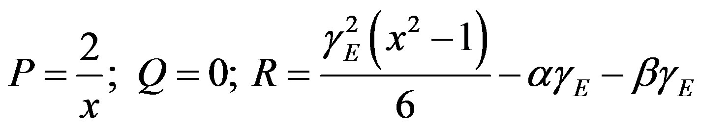
where P, Q, R are function of x. Eq.F.4 can be simplified to
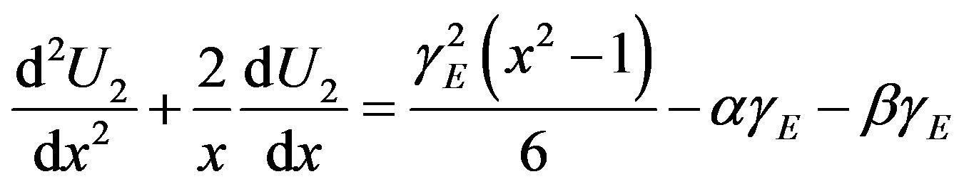 (G.2)
(G.2)
Using reduction of order, we have
 (G.3)
(G.3)
Let
 (G.4)
(G.4)
Substitute (G.4) in (G.1), if  is so chosen that
 (G.5)
(G.5)
Substituting the value of P in the above Eq.G.5 becomes
 (G.6)
(G.6)
The given Eq.G.2 reduces to
 (G.7)
(G.7)
where
 (G.8)
(G.8)
Substituting (G.8) in (G.7) we obtain,
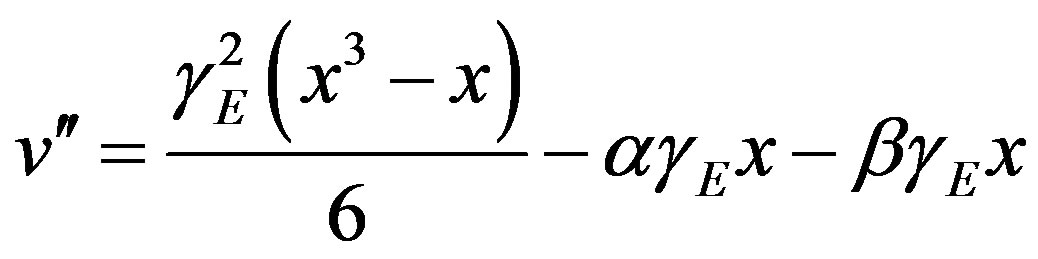 (G.9)
(G.9)
Integrating Eq.G.9 twice, we obtain
 (G.10)
Substituting (G.6) and (G.10) in (G.4) we have,
 (G.11)
Using the boundary conditions Eqs.F.6 and F.7, we can obtain the value of the constants A and B. Substituting the value of the constants A and B in the Eq.G.11 we obtain the Eq.F.10. Similarly we can solve the other differential Eqs.B.11, D.4-D.6, F.3 and F.5 using the reduction of order method.
APPENDIX H
Scilab/Matlab Program to Find the Numerical Solution of Eqs.7-9
function pdex1 m = 2;
x = linspace(0,1);
t = linspace(0,100);
sol = pdepe(m,@pdex1pde,@pdex1ic,@pdex1bc,x,t);
u = sol(:,:,1);
surf(x,t,u)
title('Numerical solution computed with 20 mesh points.')
xlabel('Distance x')
ylabel('Time t')
figure plot(x,u(end,:))
title('Solution at t = 2')
xlabel('Distance x')
ylabel('u(x,2)')
% -------------------------------------------------------------function [c,f,s] = pdex1pde(x,t,u,DuDx)
c = 1;
f = DuDx;
r=10;
alpha=5;
beta=2;
s = -r*u/(1+alpha*u+beta*u*u);
% -------------------------------------------------------------function u0 = pdex1ic(x)
u0 = 1;
% -------------------------------------------------------------function [pl,ql,pr,qr] = pdex1bc(xl,ul,xr,ur,t)
pl = 0;
ql = 1;
pr = ur-1;
qr = 0;
APPENDIX I
Determining the Region of h for Validity
The analytical solution should converge. It should be noted that the auxiliary parameter h controls the convergence and accuracy of the solution series. The analytical solution represented by Eq.11 contains the auxiliary parameter h, which gives the convergence region and rate of approximation for the Homotopy analysis method. In order to define region such that the solution series is independent of h, a multiple of h-curves are plotted. The region where the distribution of  and
and  versus h is a horizontal line is known as the convergence region for the corresponding function. The common region among
  and its derivatives are known as the over all convergence region. To study the influence of h on the convergence of solution, the h-curves of
  and
and  are plotted in Figures 2(a) and (b) respectively, for
 . These figures clearly indicate that the valid region of h is about (−2 to −0.5). Similarly we can find the value of the convergence control parameter h for different values of constant parameters.
APPENDIX J
Nomenclature
Symbols
 : Substrate concentration (mmol∙dm−3)
 : Phenyl acetate concentration (mmol∙dm−3)
 : Substrateinhibition constant (mmol∙dm−3)
 : Michaelis-Menten constant (mmol∙dm−3)
 : Kinetic parameter (mK)
 : Particle radial co-ordinate (None)
 : Dimensionless substrate in the biofilm (None)
 : Diffusion coefficient (dm2∙s−1)
 : Saturation parameters (None)
 : Dimensionless distance (None)
 : Dimensionless concentration (None)
 : Reaction diffusion parameter (None)