Natural Science
Vol.5 No.2A(2013), Article ID:28354,14 pages DOI:10.4236/ns.2013.52A039
Relative importance of different physical processes on upper crustal specific heat flow in the Eifel-Maas region, Central Europe and ramifications for the production of geothermal energy
![]()
Institute for Applied Geophysics and Geothermal Energy, E.ON Energy Research Center, RWTH Aachen University, Aachen, Germany; *Corresponding Author: Lydia.Dijkshoorn@agentschapnl.nl
Received 21 December 2012; revised 20 January 2013; accepted 6 February 2013
Keywords: Crustal Heat Flow; Physical Process Modeling; Eifel; Geothermal Energy; Hydrothermal System
ABSTRACT
We study the recent upper crustal heat flow variations caused by long-term physical processes such as paleoclimate, erosion, sedimentation and mantle plume upwelling. As specific heat flow is a common lower boundary condition in many models of heat en fluid flow in the Earth’s crust we quantify its long-term transient variation caused by paleoclimate, erosion or sedimenttation, mantle plume upwelling and deep groundwater flow. The studied area extends between the Eifel mountains and the Maas river in Central Europe. The total variation due to these processes in our study area amounts to tectonic events manifested in the studied area 20 mW/m2, about 30% of the present day specific heat flow in the region.
1. INTRODUCTION
Studying the variation of crustal temperature and vertical specific heat flow is important for the interpretation of the recent thermal regime. The variation is caused by different physical processes and is important for assessing the long-term behavior of thermal power and temperatures of geothermal energy. Often a constant vertical specific heat flow q is taken as basal boundary condition for 3D heat and fluid flow models. We use a 3D model to perform sensitivity analyses with respect to different physical processes and study their effects on the longterm variation of specific heat flow and temperatures. Using 3D transient models we quantify contribution of different geologic and tectonic process acting over years on transient thermal regime. In particular, we study the effects of extension, erosion or sedimentation, water flow, paleoclimate and deep magmatic processes such as the upwelling of the Eifel plume. These processes are quantified with respect to their thermal response period and there contribution to the present specific heat flow.
First we describe the geology of the study area, then the physical processes and their associated effects on transient specific heat flow follow. These are quantified using 1D, 2D and 3D models to determine the thermal response time and to account for heterogeneity in thermal and hydraulic conductivity. The generic of 2D crosssection models are conductive and do not account for topography. The 3D model is based on measurements, maps, and deep balanced profiles.
To use a methaphor, if we drop a stone into the water, a little later the effect is gone, but if we have a tsunami the effect is much larger and longer. Similarly, if a sudden temperature change occurs at a surface of a infinite half layer, the thermal diffusivity (“thermal velocity”) into the earth is very slow; changes of a million years ago, which remained a large period (1000 years) can still have an effect on the present deep borehole temperatures. Contrary, temperature changes with a short time period, like day and night, have only a very shallow effect. To show this, a responce time [1]. The red circle indicates the study area curve is presented from each geologic phenomena.
2. THE EIFEL-MAAS REGION
Our study area extends across the borders of Belgium, the Netherlands and Germany. It is bordered to the North by the Brabant Massif, to the South by the Eifel-Venn Massif, to the East by the Rur Graben and to the West by the Maas. The area forms the front of the Variscan orogenic belt in Northwestern Europe, which experienced erosion during the Permion to Triassic periods. At present the Eifel-Venn Massif, as part of the Rhenish Massif, forms an elevated plateau up to 700 m elevation. The study area lies at the Variscan front between the river Maas and the Eifel-Venn Massif (red circle in Figure 1).
Geological History
To give an insight in the geological history of the formation of Eifel and foreland Stratigraphical sequences, a chronological reconstruction of geological processes as synthesis of current ideas is presented.
In the Silurian (Figure 2), 420 Ma B.P., Avalonia moved to the North, resulting in a collision between Baltica, Avalonia and Laurentia, known as the Caledonian orogenese. The crust is compressed, so large mountains are formed, and Baltica slab is subducted underneath the Avalonian crust. This slab is quickly heated, resulting in upwelling of hot mantle magma. The Caledonial orogen; now known as the Brabant Massif, is a large anticlinal structure with a W-E direction; with Cambrian rocks in the center and Ordovician to Silurian rocks at the flanks. The total thickness of these rocks is about 7000 m [2]. Old Silurian Vulcanic belts lie at the Southern border of the Brabant Massif and at Visé, 20 km S-W of Aachen. The volcano’s have dacitic (63% - 68% of SiO2) and rhyolitic (68% - 78% of SiO2) deposits and therefore belonged to the most explosive category [3,4].
The volcans might be caused by a granitic batholite. This body is interpreted as the product of the melting of siliceous crust induced by continent-continent collision, and Precambrium rocks (72% of Gneis). Geophysical interpretations of gravity anomalies suggest a granite intrusion at a depth of 1 km to 5 km. A study near of the granite intrusion shows pegmatites enriched in gold,
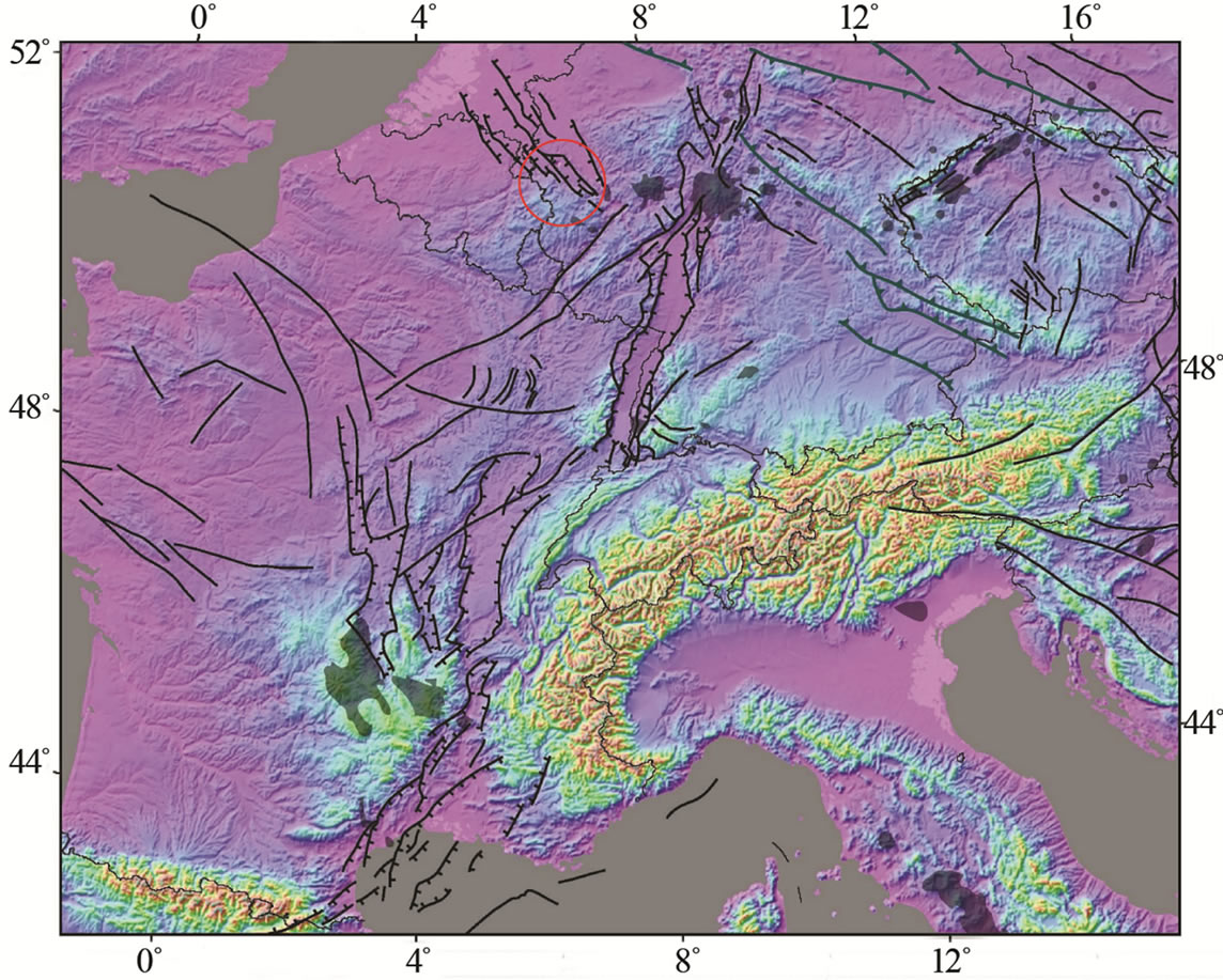
Figure 1. Digital elevation model of the European Cenozonic Rift System with superimposed fault systems [1]. The red circle indicates the study area.
wolframite and tin and at a larger distance sulphides with copper, zinc, lead, silver, molybdenum.
The Bilzen magnetic high in the Northwest may reflect either the pre-Silurian basement of the Brabant Massif, or an old intrusion of possibly (pre) Variscan age [5].
During the Devonian (Figure 3) to Carboniferous (416 - 359 Ma B.P.), the huge mountains of the Brabant Massif are eroded and uplifted. Their sediments filled the existing southern ocean (see Figure 3). The sediment thickness of Devonian to Carboniferous age increases in southern direction [6]. See reconstruction profile of the Brabant Massif in southeasterly direction (Figure 4).
During the process of erosion and sedimentation there were small sea level variations [7]. The part of the Brabant Massif is only covered with middle Devonian Frasnian deposits [7]. In the early Devonian and the late Devonian, it was above sea level.
At a later stage, during the Carboniferous Figure 5 Westfalian (315 Ma. B.P.), the Gondwana continent in the South moves northward forwards to Avalonia. This
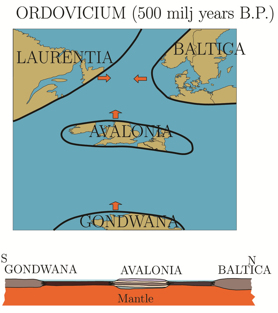
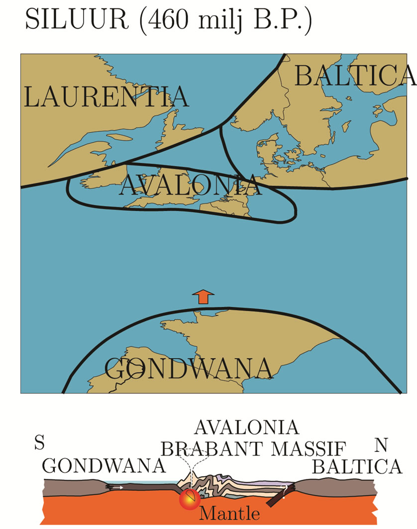
Figure 2. Ordovicium and Silurian.

Figure 3. Paleo-relief during Devonian [8].
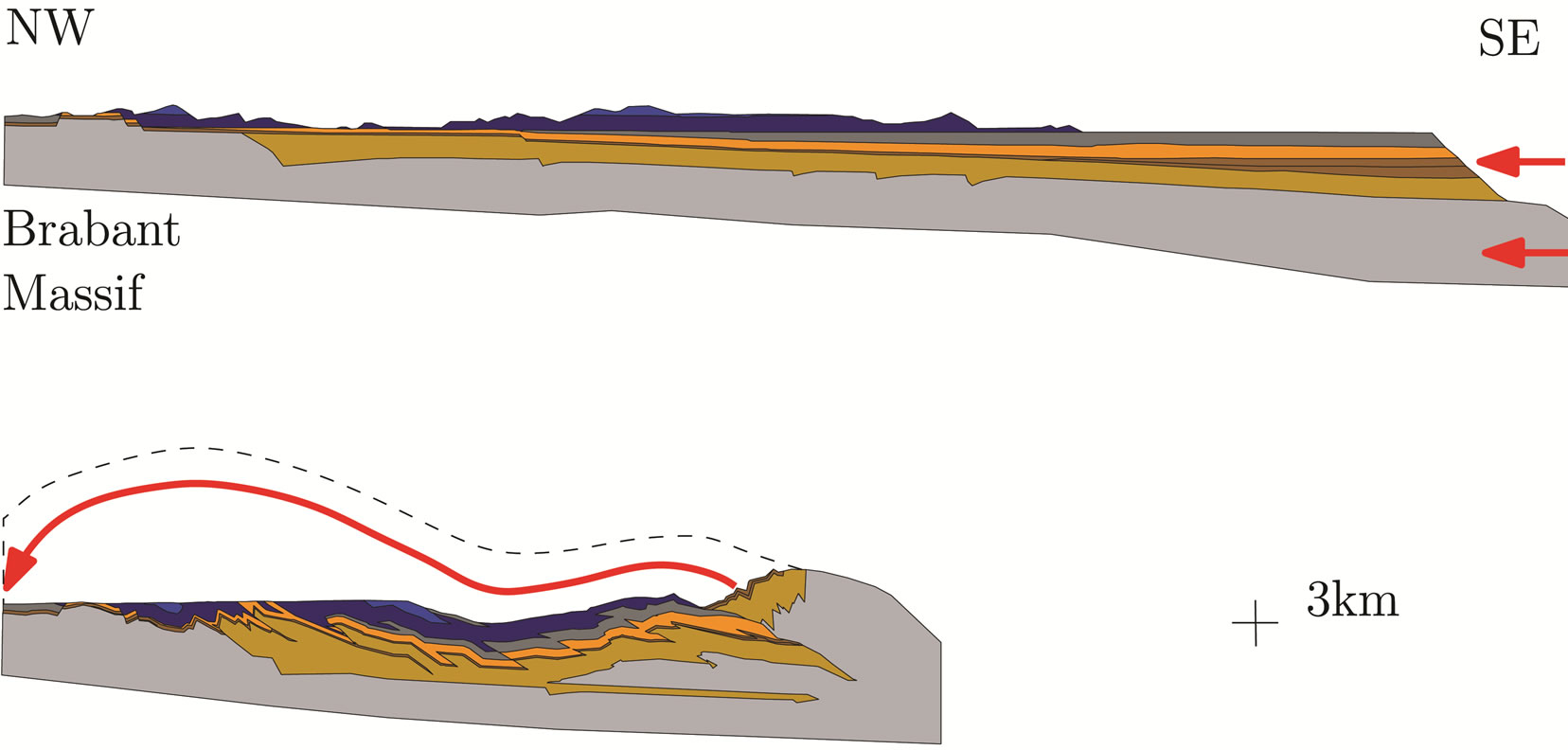
Figure 4. Paleo-relief during Devonian and Carboniferous [8] and cross section during late Carboniferous [6].
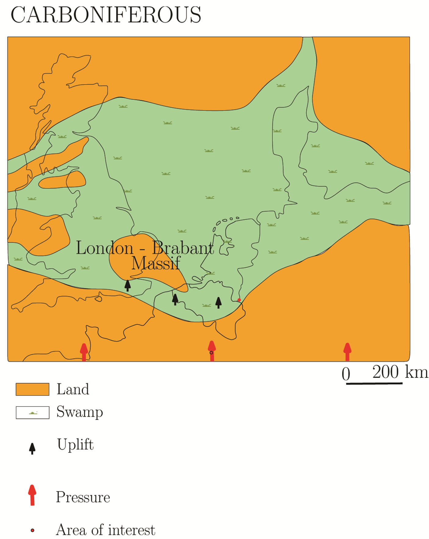
Figure 5. Paleo-relief Carboniferous [8].
causes a shortening of the crust and a faster subduction of the basin with accordingly large deposits.
Large swamps are formed, with a luxuriant vegetation at the equator. Note that the Brabant Massif was totally covered with carboniferous sediments. Studies indicate that one meter of present coal thickness corresponds to 25 m of organic deposited material. Dead plants were covered relative fast by sediments, consequently there was too little oxygen to degrade them. The water and formed gas could not escape due to the fast subduction and due to the low permeability of peat and shale. This results in a very thick Carboniferous swamp with verymud water and high gas pressure and temperature. The latter is caused by the very low thermal conductivity of gas, water and peat: low thermal conductivity causes the temperature gradient to increase. These large swamps correspond to today’s large coal mining regions.
During the late Carboniferous, Gondwana moved to the North resulting in an arc-continental collision of Gondwana with Avalonia, known as the Variscan orogeneses. [9] studied this orogeneses numerically using different models. All models indicate that the crustal root formation, delineation, and hot asthenosperic heat advection might have occured within 1 Ma - 10 Ma period.
Due to this collision large mountains were formed again Figure 4. In the study area—Eifel-Maas, Brabant Massif—more phases of this orogenic stage can be distinguished.
Firstly, deeper parallel overstrusted faults developed between the Namurian and the Westfalian B periods. Secondly, a large sheet overthrust, eroding the Carboniferous sediments and forming a sheet overlaying the older formations. A reason for travelling this long distance might be the large, over-pressured Westfalian swamp; high temperature and high fluid pressures provide small resistance to external stresses. When a dense sheet loads on a low density swamp with high fluid pore pressure, the warm water and gas is squeezed out, resulting in the large fluid flow at the front of the Variscan reported by [10,11].
The overthrust sheet partly removes the original Westfalian and Namurian sediments deposited them as huge mountain over the Brabant Massif in the Northeast. High vitrinite reflections [5] at the northeastern side of the Brabant Massif support this scenario. Models performed at the Netherlands suggest a cover of at least 2700 m [8] in post-Westfalien C age. During the Permian period, 280 Ma B.P., all continents together formed the so-called super continent Pangea with a very low sea level. The area which currently lies at the North Sea, but at that time laying near the equator was drying, which formed large and thick Salt layers.
Between the Permian and the Triassic period (251 Ma B.P.) 90% of all marine species and 70% of all terrestrial species died.
During the Triassic and Jurassic period (251 Ma - 145 Ma B.P.) the large mountains (i.e. the Brabant Massif in today’s Belgium), erodes filling the oceans with sediments. In the study area, no Triassic or Jurassic sediments were deposited.
During the late Cretaceous, the Supercontinent Pangea split up into the present American and European plates separated by the Atlantic Ocean. At that time the sea level was about 100 m to 300 m higher than the present sea level. Hydrothermal precipitation formed sulphide ore deposits during the early inversion of the Rhine Graben in the Cretaceous. The deposits occured mostly in the Dinantian chalk, but also in the under Cretaceous limestones, consisting of zinc and lead. The Rur Graben was reactivated and several SW-NE striking faults were formed in an area presently marked by a prominent gravity low.
In the Tertiary 45 Ma B.P., volcanic eruptions occurred in the Eifel mountains. Two new volcanic fields evolved during the Quaternary last 600 ky with the last eruptions only 11 ky - 12 ky B.P. At the same time the Rhenish Shield experienced strong uplift of the (up to 250 m in 600 ky). This uplift is an isostatic response of the lithosphere to a deepseated buoyant hot body. This hot body was detected by seismic tomography [12] and is known as the known Eifel mantle plume.
The volcanic deposits are dominated by potassiumrich, mafic (Mg-Fe rich) minerals, poor in silica. Larger peridotite xenoliths occur, which are typical for intraplate, continental settings. Many xenoliths originate from lower crustal and upper mantle sources. The Western Eifel volcanic field is about 600 km2 in area and contains around 240 individual volcanoes. The Eifel volcanic region is associated with the Rhine Graben, a continental rift zone. The Rhine Graben became active during the Eocene, and fault movements intensified during the Miocene. Since the Miocene, the tectonic activity of the Rhine Graben and other rift zones of western Europe have continued at a lower level minor fault movements, with occasional small earthquakes, and Quaternary volcanism in Eifel.
3. SELECTED DATA FROM PUBLICLY AVAILABLE SOURCES
A lot of study has already been done in the area. So I present you the available information of these studies, and discuss their relevance to model.
3.1. Geologic Maps and Profiles
Different geologic maps exist in the three countries: 1) Current subcrop geological maps are available from the different geological surveys; 2) Older geological maps exist which contain the depth of different geological units. They were compiled by a collaboration between the three countries during the coal exploration period. Table 1 gives an overview of the available geological maps, the country, and the reference.
The different geological maps as well as the depth
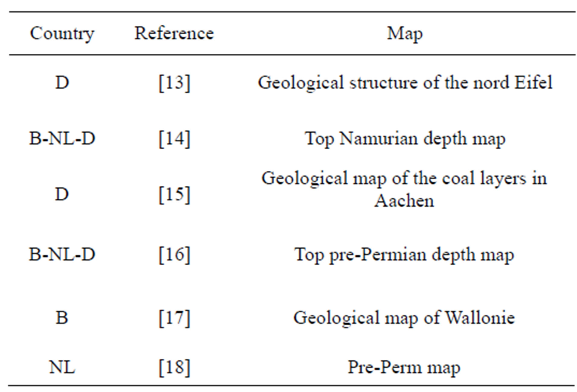
Table 1. Overview of geologic maps of different countries with references used for modelling (with B: Belgium, NL: The Netherlands and D: Germany).
maps of the different layers were digitized for use in a 3D model. The maps of the different countries are based on three different coordinate systems. [16] matched his maps together by eye, so some errors were inevitable Since the largest part of the model is on Germany we choose the common used German coordinate system; Gauss-Kruger. The final result, a combined geological map of parts of the three countries is shown in Figure 6.
The map shows a large synclinal basin with Devonian subcropping layers in the South. In the North, there is an anticline enclosed with carboniferous layers. The Aachen Overthust separates the two parts. The pre-Perm geological layers where eroded during millions of years, creating a very smooth and flat surface dipping to the north. Discordantly on top of this surface the Cretaceous limestone layers were deposited, with thickness increasing to the North. It can be clearly seen that the faults related to the Rhine Graben where later reactivated and changed the smooth top pre-Perm surface during later periods, which became subsided in different blocks towards the graben.
![]() Seismic lines in the study area are sparse. The deep DEKORP line [19,20] was used to construct two balanced parallel profiles; Profiel of Winterfeld [10] and Profile of Hollmann [6].
Seismic lines in the study area are sparse. The deep DEKORP line [19,20] was used to construct two balanced parallel profiles; Profiel of Winterfeld [10] and Profile of Hollmann [6].
The Profile of Hollmann is not only based on the information from the DEKORP line but contains also information on geologic enclosures along the Maas river and information from the deep boreholes Boland and Soumagne. These boreholes provide more constraints for the profile. It has a depth of 5 km and a length of 60 km.
The profile Winterfeld does not include information from deep boreholes, why it is only constraint on its upper part, which is based is based on dips and subcrops of the different geological layers. Considering the fact that the dips are steep, the subcropping layers can be extrapolated to larger depths and provide much more information about the geology at depth than, for example, a flat laying layer would do. Comparing the two profiles it is quite clear that it is impossible to fit them easily into a 3D geological model. Especially the deeper part, the lower devonian is totally different in the two different profiles. The description of the forming process of the profiles is equal, namely the shortening of the crust during the late Variscan orogenese due to overthrusting. The way the overthrusting is explained differently way. This makes it impossible to extrapolate the geological layers between the two profiles.
In the region bounded by the Hollmann and the Winterfeld profiles, there are more profiles from [17] providing some valuable information on the subcrops and dips of the geological layers. The location of all of the profiles are shown in Figure 6 from West to East; The Hollmann profile [6], the four extented geology profiles [17], the
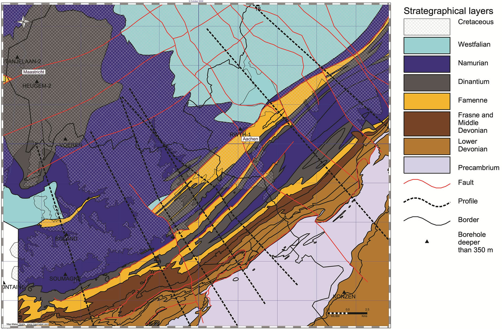
Figure 6. Location of geology and faults, the boreholes, profiles, large cities and borders.
Winterfeld profile [10] and the Steinkohle profile [15].
3.2. Magnetotellurics
[21] analyzed the electromagnetic data from the Eifel region, which were collected from 30 stations during campains in 1997 and 1998. They covered an area of about 140 km by 130 km. A 1D model suggests a layer of highly electrical conductivity layer at a depth between 15 km and 25 km in the lower crust. Despite its still unknown origin, [21] states this as a very common phenomenal. He also performed a 3D model inversion. The results of the 3D model are shown in Figure 7. Layer 2 between 14 km - 22 km depth has high electrical conductivity vertikal units alterations with low conductivity units. Possible causes are saline water, graphite, Fe/Tioxides, sulphide.
3.3. Earthquake Tomography
To study the crustal and mantle structure of the intraplate volcanic fields and their deep origin, a network of 84 permanent and 158 mobile seismographic stations was set up [12,22]. Schematic overview of the principle of tomography is shown in Figure 8.
To calculate a S wave velocity reduction tomogram 3773 residuals are used. From the travel time anomaly [12] estimated an excess temperature of 200 K - 300 K for a plausible plume in the uppermost 100 km of the mantle, where 1% of partial melt reduces this temperature with about 100 K. According to [12] teleseismic P-wave attenuation shows a strong absorption anomaly in the lithosphere and a weaker anomaly in the mantle, and the lithospheric anomaly is interpreted as scattering attenuation at a magmatic intrusion zone. In the asthenosphere temperature induced solid-state anelastic attenuation is assumed. The Pand S-velocity anomalies in the lithosphere and upper asthenosphere can be explained by an increase of temperature by about 100 K - 150 K plus 1% of melt. The Eifel plume anomaly is spread out above the 410 km depth discontinuity and rise up mainly beneath the Eifel [22] and the massif Central [23]. In Figure 9 a small extension at the top of the plume can be seen in the NNW direction underneath the Roer Valley Graben and our study area.
3.4. Gravity
Figure 10 shows the gravimetric anomaly map [24] in the region. The station density varies from 1 per 80 km2 to 2.5 per km2 (e.g. Brussels area). The anomalies are calculated using a uniform Bouguer reduction density of 2.67 g/cm3.
The negative anomaly into the Roer valley graben, indicate a shorten of weight because of the less dense layers of Quaternary, Tertiary and Cretaceous age. To the northwest a shorten of weight is due to the less dense Jurassic and Triassic sediments. The crustal stretching model of MacKenzie, shows that less dense mantle material will attempt to flow to this area to compensate the gravity anomaly; like communicating vessels, but slower.
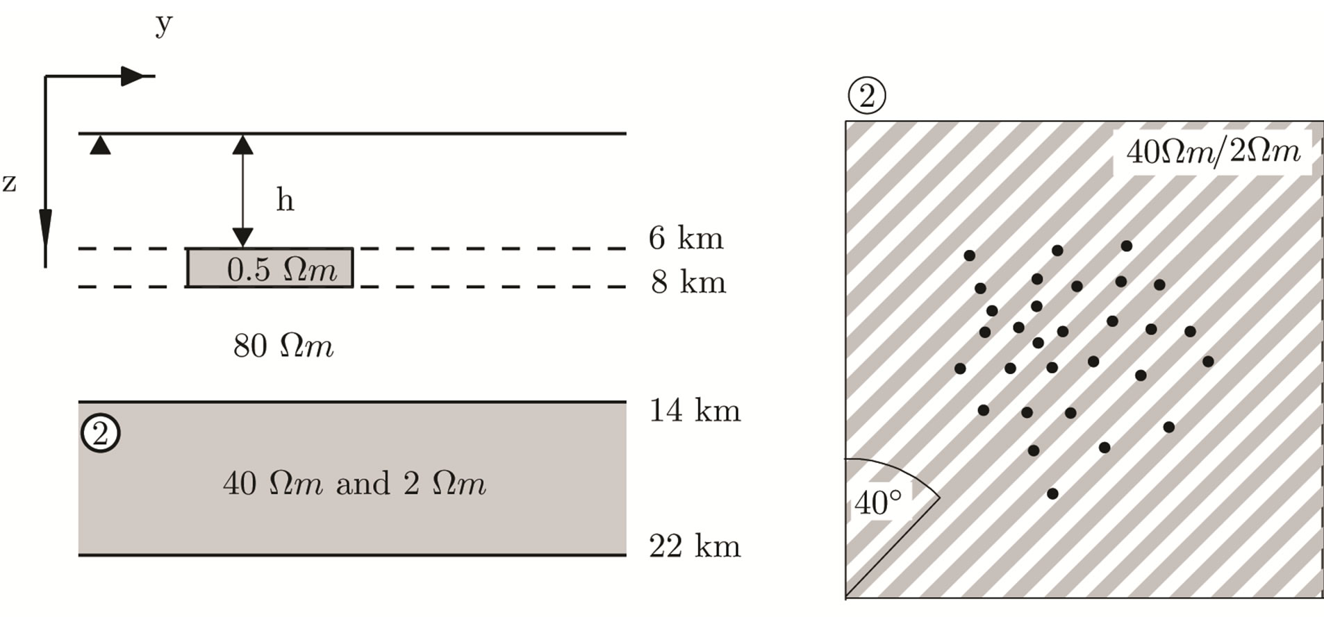
Figure 7. Magnetotelluric model [21], profile [6], the four extented geology profiles [17], the Winterfeld profile [10] and the Steinkohle profile [15].
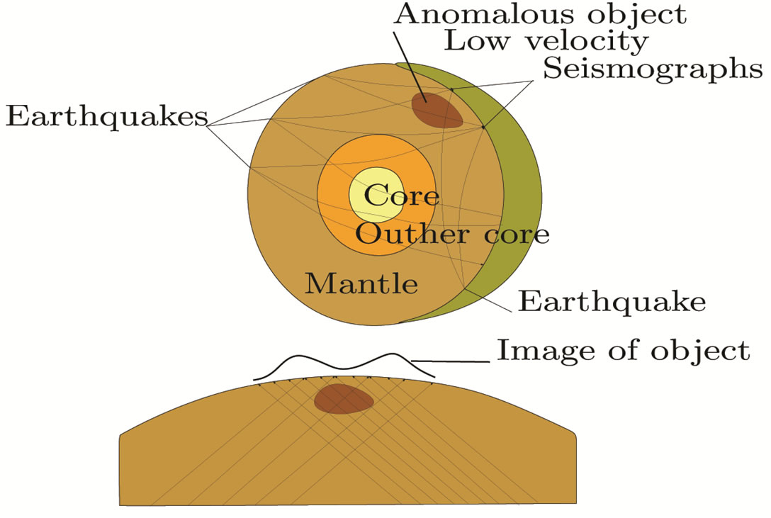
Figure 8. Schematic overview of the principle of tomography. Due to the slow velocity and attenuation of the anomalous object, the arrival times increases when the wave passes the object. Inversion of the signal gives the borders and the properties of a-nomalous object.
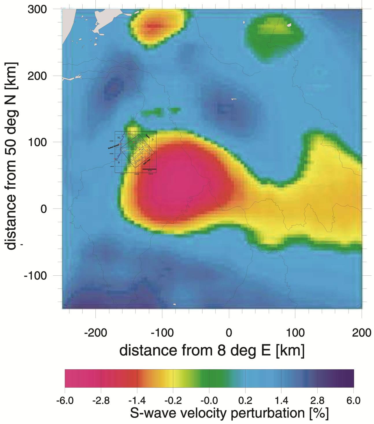
Figure 9. S-wave tomogram of Eifel plume model [12] for the interval from 31 to 100 km depth with the 3D model boundaries presented in this paper and the main faults in the model area.
This fits with results of the S-wave tomogram, where the low velocity layer indicate the presence of a mantle plume front underneath the Roer valley graben. The rift Roer valley graben can be seen as the first stage of the Wilson cycle [25,26]. According to this theory it will
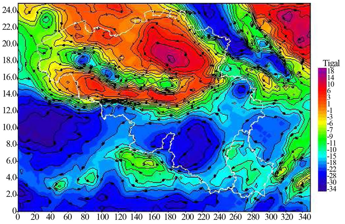
Figure 10. The bouquer anomaly in Belgium and surroundings
[24].take 12.5 Ma before the astenosphere rises the surface.
3.5. Vitrinite Reflections
Vitrinite reflection measurements on of organic material like peat, lignite or coal can be used to declare a maximum temperature. Vitrinite reflections R0 near the Brabant Massif vary between 2% and 5%. According to [27], who performed 600 vitrinite reflection measurements, time is not important for determining the maximum temperature Tmax from vitrinite reflections. They proposed a relationship:
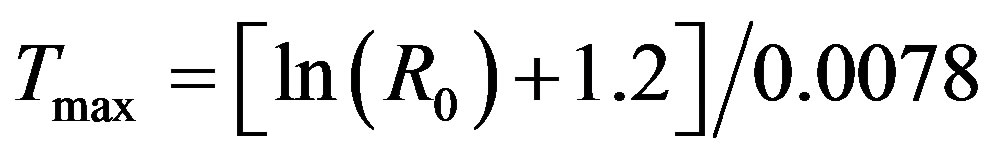 (1)
(1)
Table 2 shows their maximum temperature Tmax for different vitrinite reflections R0 .
3.6. Thermal Springs
The study area is famous since Roman times because of its hot springs (200 m). The water circulates from the high Eifel-Venn Massif (700 m) to the lower where it ascends in the thermal springs situated in Aachener and Burtscheid. These springs have a total flow rate of 175 m 3/h, a maximum temperature of 79˚C and an average temperature of 60˚C [28]. Geothermometers [29] were used to determine the composition of the thermal waters [28] and to determine the average temperature. Geothermometers also provide information on the maximum temperature during the residence period of the geothermal water. [29,30] calculated the mean subsurface temperature. Table 3 summarizes the result for the different geothermometers.
The geothermal spring water shows a high concentration of CO2 180—mg/L of dissolved CO2 gas, this is typical for geothermal systems. They are located in areas of higher CO2 flux, due to the particular geological structures that give origin to a geothermal reservoir. Much higher CO2 fluxes are found in volcanic areas. A larger amount of natural CO2 is produced at depth, mainly by thermo-methamorphism of marine carbonate rocks. This CO2 is usually trapped in deep structures, saturates the deep aquifers and it is discharged at the surface through natural manifestations and soil degassing. Degassing CO2 from more than 90 M Pa results in a temperature increase due to expansion, from less than 90 M Pa the temperature decreases due to expansion. [28] did some calculations with computer program SOL-MINEQ.88 and stated that formation water, which is normally in equilibrium with calcite and temperatures of 120˚C until 135˚C before rising, has a pH of 5.8 - 6 and a CO2 concentration 1000 mg/L, so it is highly saturated in calcite. When the water rises to the surface it is cooling, the pH increases and calcite precipitates. In this process the dissolved CO2 is used for forming CaCO3, which results in a decrease of the CO2 concentration of the water to about 200 mg/L. The geothermal water of the springs is meteoric water and has a residence time of more than 20000 years.
[31] described the Benzenrade fault located to the north of Aachen. Between 1923 and 1955 several mine tunnels crossed this fault. The fault had a cross thickness of about 110 m till 50 m, and consisted of quartz, pyrite, galenite, sphalerite and chalcopyrite. Thermal water springs of 50˚C were found at a depth of 640 m at 250 A (a specific historic mine tunnel) Figure 11.
3.7. Borehole and Laboratory Measurements
Measurements of thermal conductivity on cores from deep boreholes located in Belgium were performed at the University of Leuven [32,33]. Furthermore detailed geo-
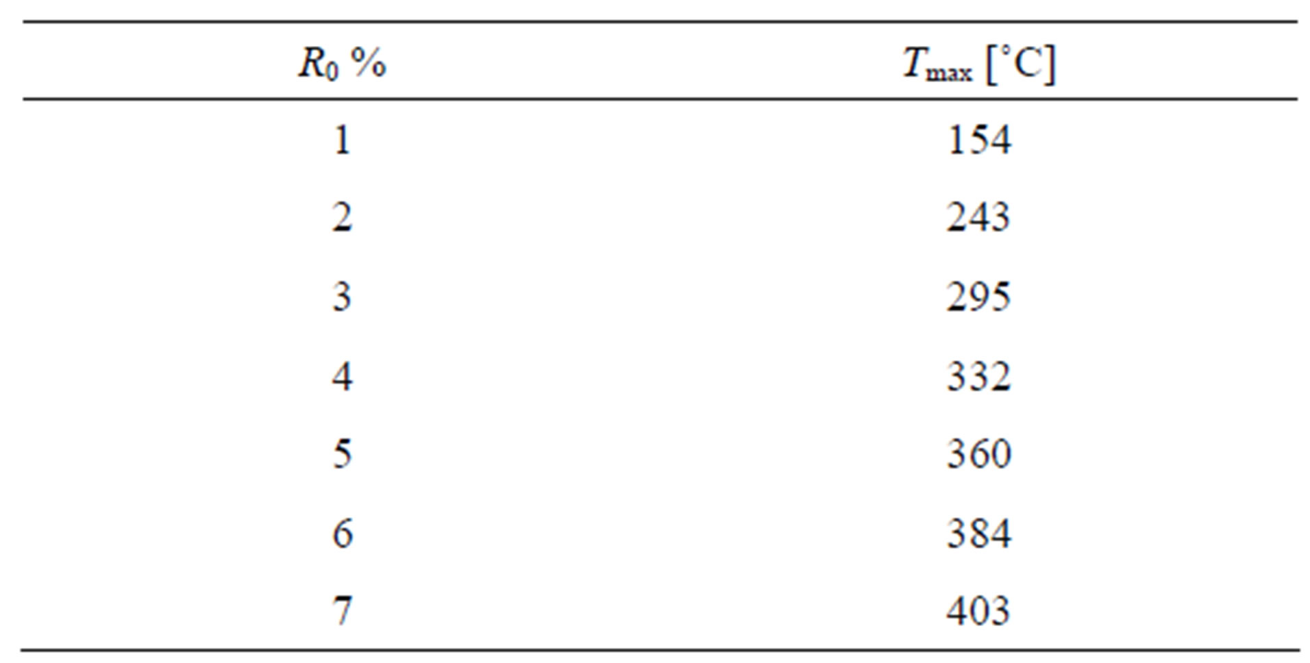
Table 2. Vitrinite reflections R0 with associated maximum temperatures Tmax according to Eq.1 [27].
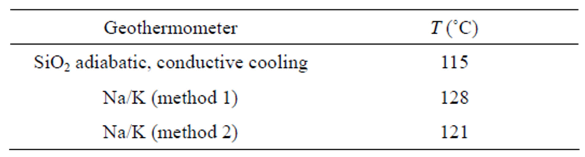
Table 3. Determination of the mean temperature from the geothermal springs using different geothermometers [29].
logical descriptions of each borehole by the Belgium geological survey, the geological survey of Netherlands and geological survey of North Rhine-Westfalia were used to collect in a database, according to stratigraphy and lithology. The position of the the boreholes are shown on the map Figure 6.
The specific gamma log of the borehole Kemperkoul was used to determine the radiogenic heat generation rate within the Namurian and Westfalian [34].
4. PHYSICAL PROCESSES AND THEIR EFFECTS ON SPECIFIC HEAT FLOW
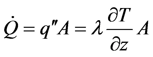
Different tectonic and geological processes have an effect on the vertical specific heat flow and the temperatures in the earth crust. This is important since these are the main parameters effecting the thermal power and temperature deliverd by installations for the production of geothermal energy. In case of a steady state where everything is in equilibrium, Fouriers law relates specific heat flow to thermal conductivity and temperature gradient.
 (2)
(2)
with  the heat flow (W),
  the specific heat flow (W/m2) A the surface area (m2), λ the thermal conductivity (W/(mK) and z the depth (m).
In most cases a constant basal specific heat flow  is taken as boundary condition for 3D coupled heat and fluid flow models.
For an average specific heat flow of 0.08 W/m2 the thermal gradient is significant larger in case of the Westfalian, the Cretaceous or the Tertiairy where the thermal conductivity is low than in case of the Devonian layers with high thermal conductivity.
Different transient processes, however, modify the steady state thermal regime. We study particularly various geologic processes which persist over long periods (i.e. millions of years) such as extension, erosion and sedimentation, water flows, deep magmatic processes (e.g. Eifel plume), and paleoclimate. These processes are characterized with respect to their thermal response time and their influence on present specific heat flow.
First of all, two orthogonal schematic cross-sections through the area Figure 11, with the RWTH-1 borehole as crossing, are divided into tree categories with respect to there thermal conductivity: 1) the Cretaceous, Westfalian, 2) the Namurian and 3) the Devonian and Precambrium, see Figure 12.
Than the sections are modelled Figure 13 using equidistant grid nodes in horizontal and vertical direction. The properties as well as the vertical heat flux are defined in the midpoints of the gridcells, but the temperatures are defined at the upper and lower borders of the
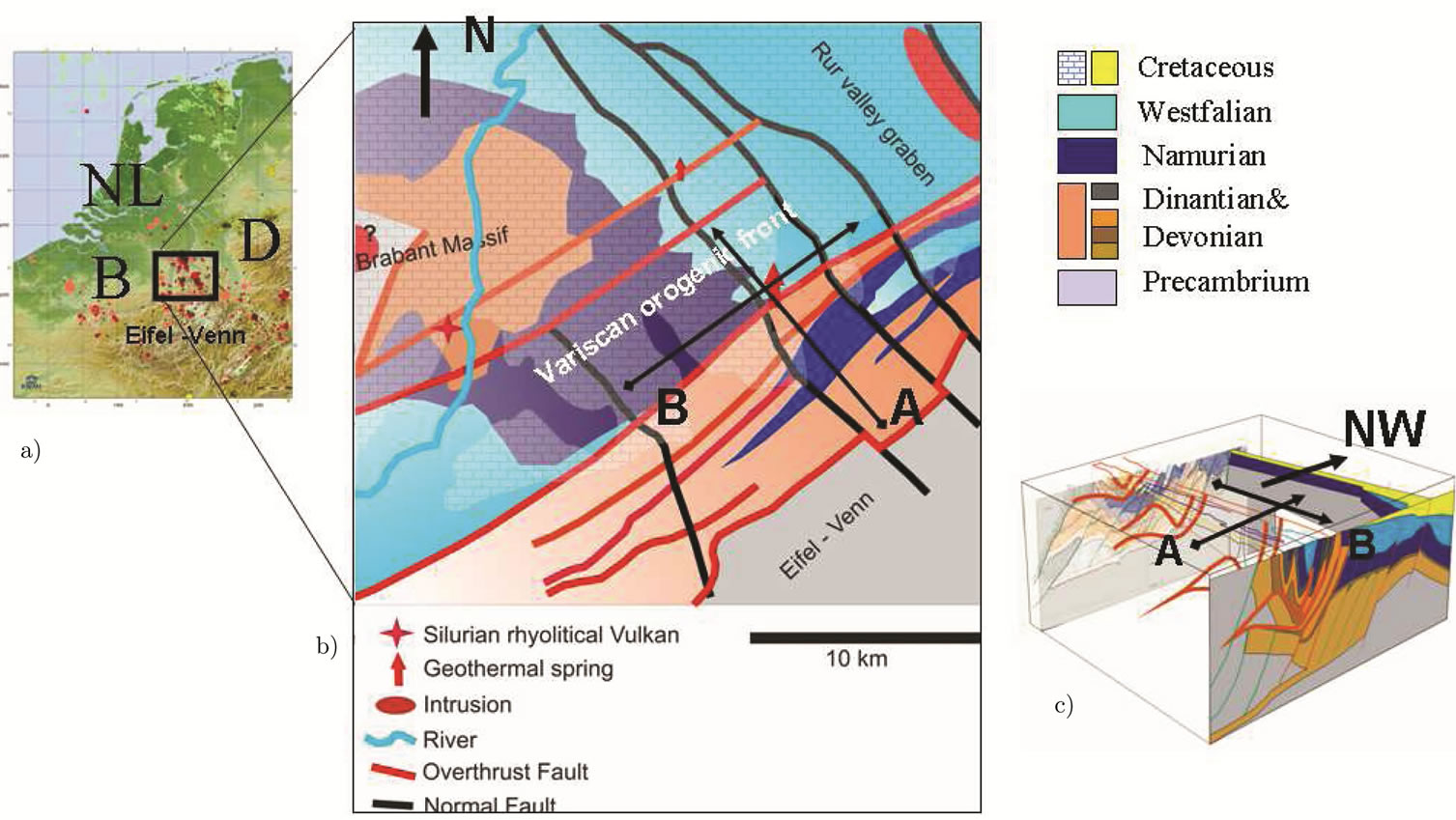
Figure 11. a) Overview map with locations of small earthquakes <3 M; b) Geologic map with geothermal springs and location of the 2D sections; c) 3D view of the stratigraphical layers with the location 2D sections indicated.
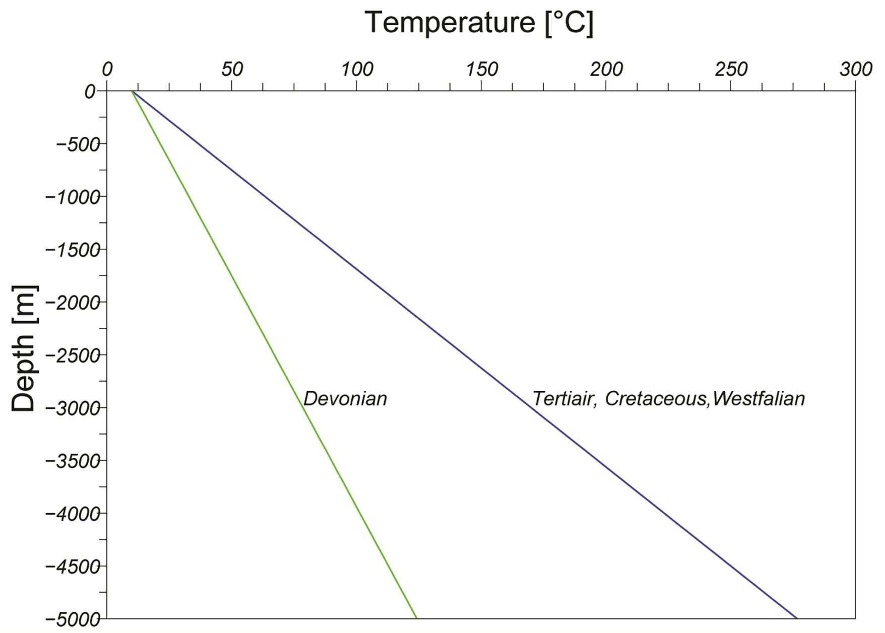
Figure 12. An specific heat flow of 0.08 W/m2 with thermal conductivity of 1.5 W/(mK) in case of the Westfalian, Cretaceous, Tertiair layers and 3.5 W/(mK) in case of the Devonian layers.
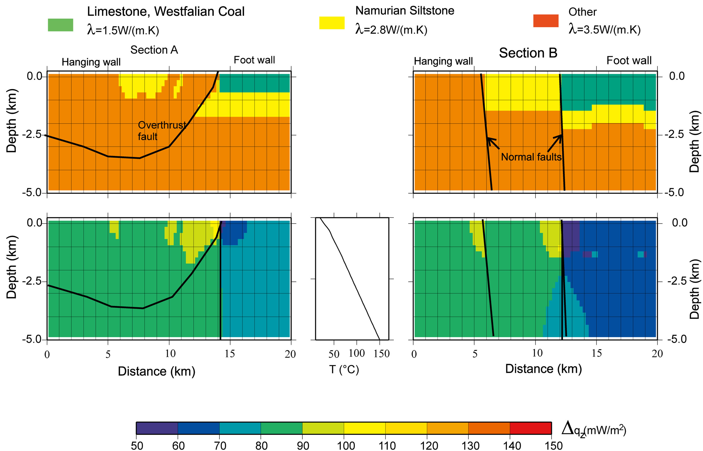
Figure 13. Two perpendicular cross sections A and B; red presents the a base temperature of 150˚C and top temperature of 10˚C. The thermal conductivity used into the model are an average of the total layer.
gridcells. Bottom temperature of 150˚C and top temperature of 10˚C temperatures are set as boundary conditions.
4.1. Erosion and Sedimentation
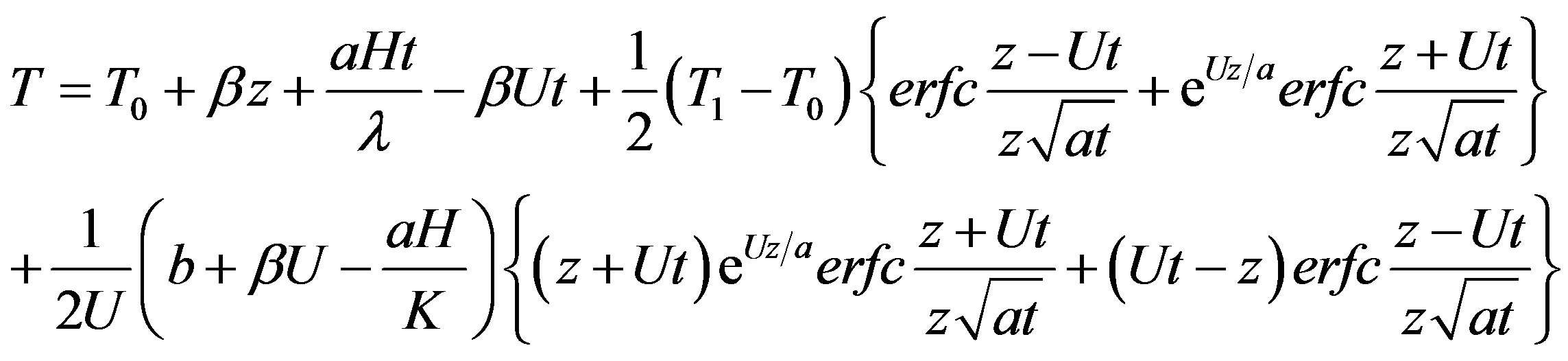
We can determine the effect of erosion and sedimentation, using the equation provided by [35, p. 388].
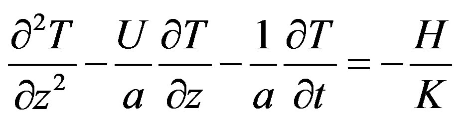 (3)
(3)
with initial condition
 with
with 
and boundary conditions
 with
with 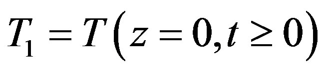
 (4)
(4)
For H = 0, b = 0 and T1 = T0
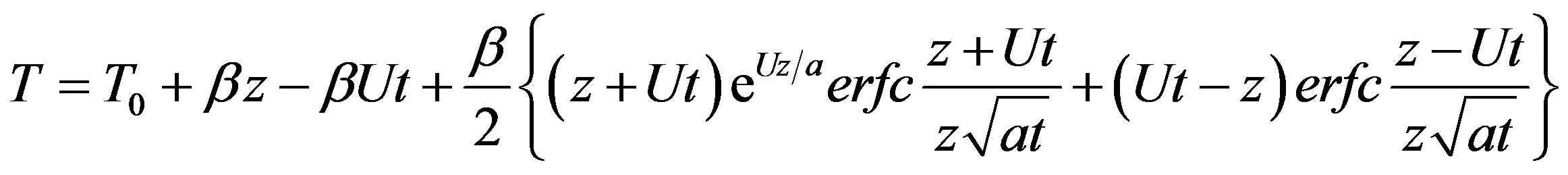 (5)
(5)
with H heat generation, a thermal diffusivity, U erosion or sedimentation rate, β temperature gradient, z the depth, and t time.
Figure 14 show the influences for different erosion rates on specific heat flow in case of no heat generation.
As described in Subsection 2.1 during million of years sediments has been deposited in the Graben and in the mean time mountains of the Brabant Massif and Eifel has been eroded. If we only consider the latest period, the Quaternary; The erosion rate could be derived from the differentiation of the different geological deposits and Maas terrace building. The rate varies between 0 mm/y and 0.1 mm/y at the hanging wall. The sedimentation rate has been calcucalculated using the quarternairy sedimentation thickness divided by the quaternary times (800,000 years). The rate varies between 0 mm/y and 0.4 mm/y at the foot wall. Using Eq.5, this yields differences of +/− 5 mW/m2 in heat flux Figure 15.
4.2. Paleoclimate
The changes in specific heat flow due to an instant change of the temperature at the surface can be written as [36]
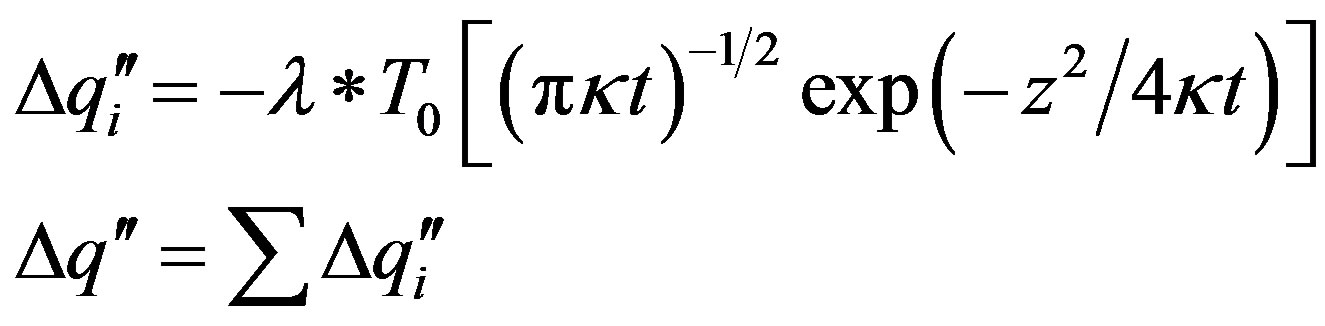 (6)
(6)
with  the specific heat flow, t the time, κ the thermal diffusivity and T0 the instant variation in temperature.
Instant variations in ground surface temperature between 10,000 years and 20,000 years B.P. yield variations in specific heat flow of zero to 9 mW/m2. The propagation of the paleoclimatic signatures with depth varies according to the different thermal diffusivity Figure 16. The paleoclimatic signature in the foot wall with Quarternary, Tertiary and Cretaceous penetrates not as deep and is attenuated stronger then in the hanging wall.
4.3. Eifel Mantle Plume
As described in Subsection 3.3 the seismic tomography suggests the hot Eifel mantle plume crossing our study area. Figure 17 shows the thermal response at a point at 5 km depth, to an instantaneous thermal pulse at a depth of 30 km [1] of a magnitude of 100˚C, 200˚C and 300˚C.
Only after 1 million year specific heat flow at a 5 km depth starts to vary reaching a peak at 10 million years whereafter it decreases again and vanishes finally. Assuming a 200 K temperature change at 30 km Moho depth Subsection 3.3, 10 million years ago, present day specific heat flow would increase by 16 mW/m2 to 17 mW/m2.
4.4. Deep Convective Water Flow
To determine the depth of the origin of geothermal water, an approach modified after [36, p. 264, Eq. 6-270].
The temperature of geothermal water changes with
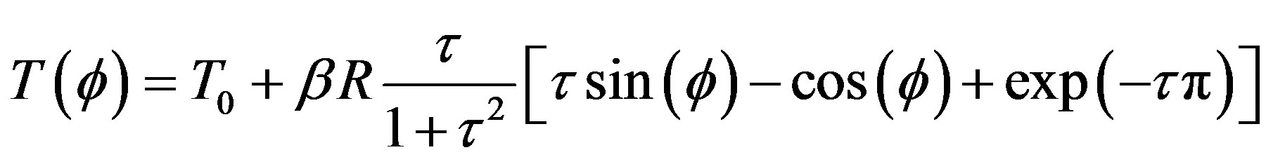 (7)
(7)
with
 (9)
(9)
Looking at the spring temperature, ( ) and assume an average thermal conductivity
 , a vertical temperature gradient
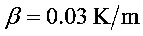 , a water infiltration temperature T0 in the Eifel of 10˚C the spring temperature is a function of the flow rate of the water Fw
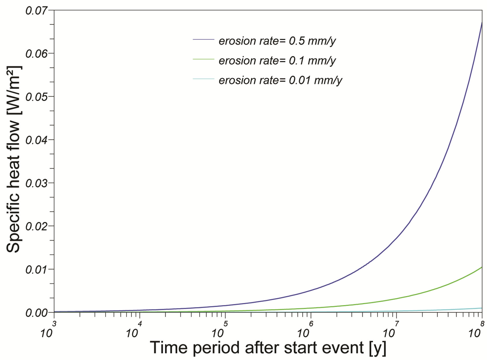
Figure 14. Thermal response curve for different erosion rates.
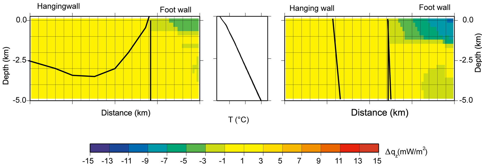
Figure 15. The relative changes in specific heat flow due to sedimentation and erosion for the two perpendicular cross sections A (left) and B (right) in the Eifel-Maas region; see Figure 11 for the location of the cross sections.

Figure 16. The possible influence of the paleoclimate on specific heat flow for two perpendicular cross sections A (left) and B (right) in the Eifel-Maas region; see Figure 11 for the location of the cross sections.
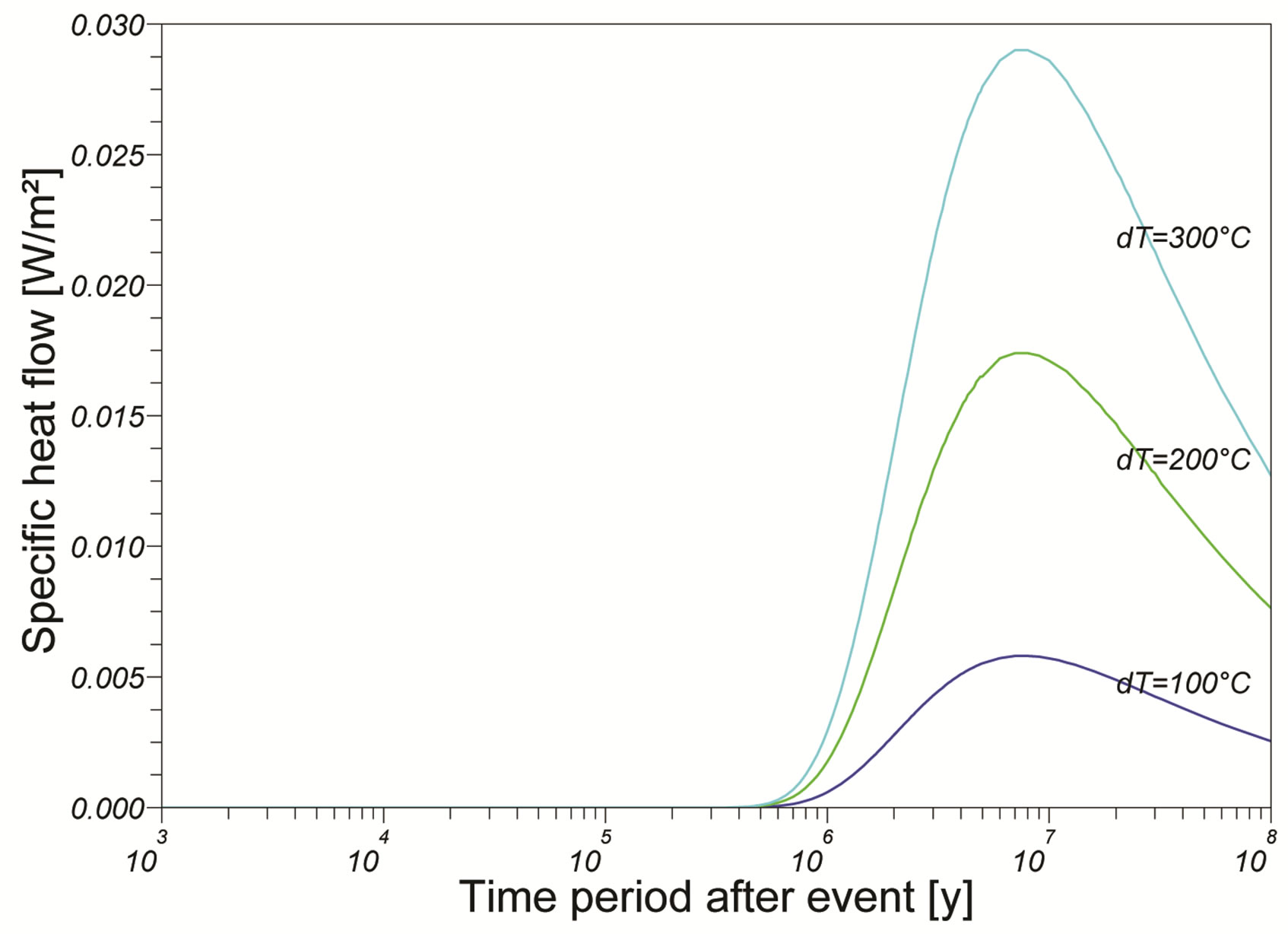
Figure 17. The thermal time response curve of a 5 km depth point for pulses with a different temperature change induced at the 30 km Moho depth.
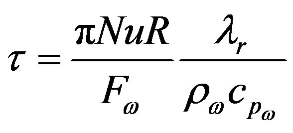
and the radius (or depth) R of the flow path Figure 18. Nu, ρw,  are respectively Nusselt number, density of the water and the heat capacity of the water. The flow rate in Aachen is known
  [28] as is the average spring temperature 60˚C. So with these parameters from Eq.8 we are able to calculate the radius R (or depth) of the flow path; which is
 . This depth is deeper than the overthrusted sheet. The maximum temperature at depth along the pathway is 130˚C see Figure 18 which agrees well with the value determined by Na/K geothermometers Table 3. The springs have been active since Roman times and probable much longer. The total thermal energy of these springs is
 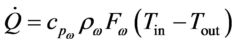 with an infiltration temperature
 , spring temperature
 , spring flow rate
 . This yields a yearly of 3.2 × 10¹¹ kW·h corresponding to a thermal power of 10.2 mW.
4.5. Joint Effect on Specific Heat Flow
The processes in the study area yield a maximum variation in specific vertical heat flow of 20 mW/m2. The hanging walls of the fault systems show increased specific heat flow due to uplift and erosion, while the foot walls show decreased specific heat flow due to down warping and sedimentation. This results in horizontal heat flow at the normal faults or the overthrust faults. Long period temperature variations at the top or bottom of the model caused by climatic changes at the surface
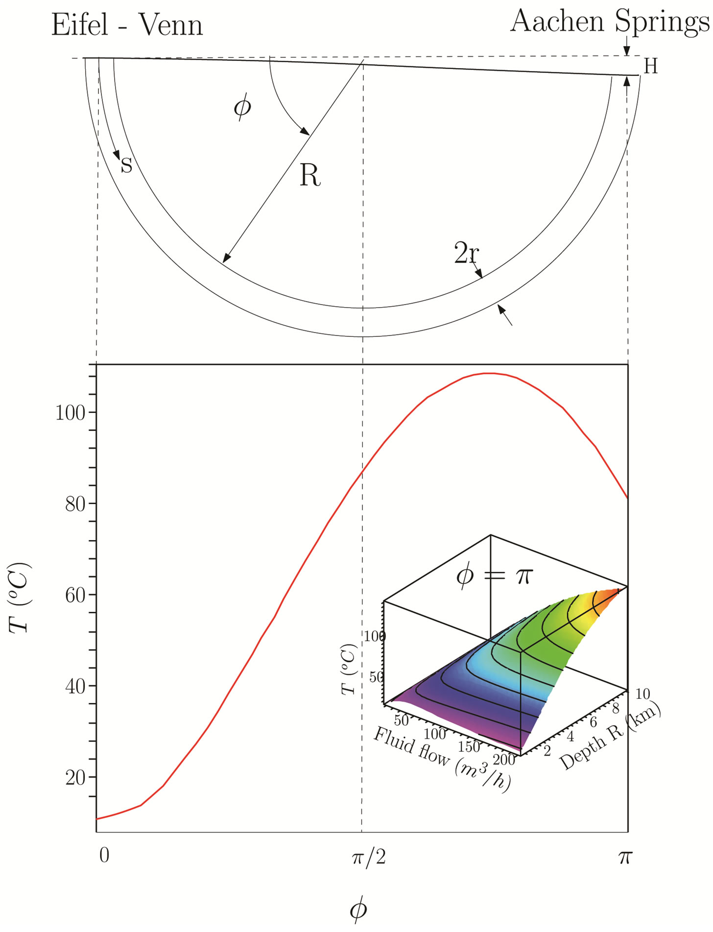
Figure 18. Schematic overview Aachener springs along there pathway, with Flow rate 175 m3/h, and an average spring temperature 60˚C [28]. The used radius R = 4500 m has been calculated with Eq.8 referred to the small 3D picture.
or deep plume yield a faster and deeper response in the hanging wall than in the foot wall. These variations are due to the higher thermal diffusivities of the older rocks in the hanging wall.
5. 3D MODEL COUPLED THERMAL AND HYDRAULIC SIMULATION OF THE EIFELMAAS REGION
Numerical 3D model simulations of coupled heat and fluid flow are used to indicate promising locations for producing geothermal heat.
5.1. Geometrical Model
To obtain a good understanding of the regional conductive and convective heat flow in the Aachen-EifelMaas region, a 3D numerical model of 40 km × 40 km × 5 km was setup for simulating heat and fluid flow. Different steps are required to set up such a model (see Figure 19): First a 2.5 D-structural model is build.
Table 4 shows a schematic overview of the stratigraphical units.
With the aid of geological maps, deep profiles and boreholes discussed in Subsection 3.1; one can reconstruct a geometrically two separate geological phenomena: 1) theolder pre-sheet overthrust faults and 2) the post-sheets for each separate normal fault block. A stratigraphical 3D model (Figure 20) is constructed by the combining of these different geometrical reconstructions.
The stratigraphical layers of the model corresponding petrophysical properties are listed in Table 4.
The model is simulated using Shemat, a finite difference code for coupled temperature and fluid flow [37]. Boundary conditions are; a surface temperature of 10˚C which is a mean of the average temperature [38] and the deep boundary temperature at 30 km of 1200˚C [1] The
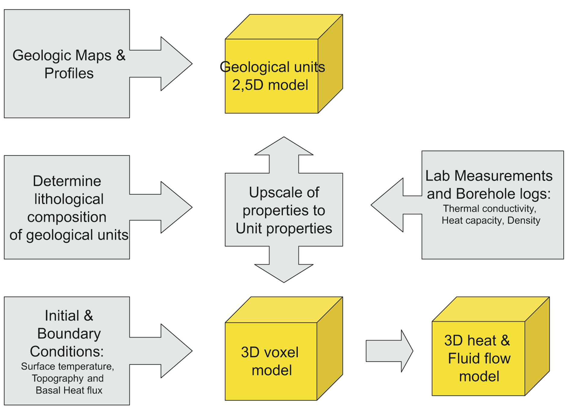
Figure 19. Flow chart to determine the input parameters for the different model units.
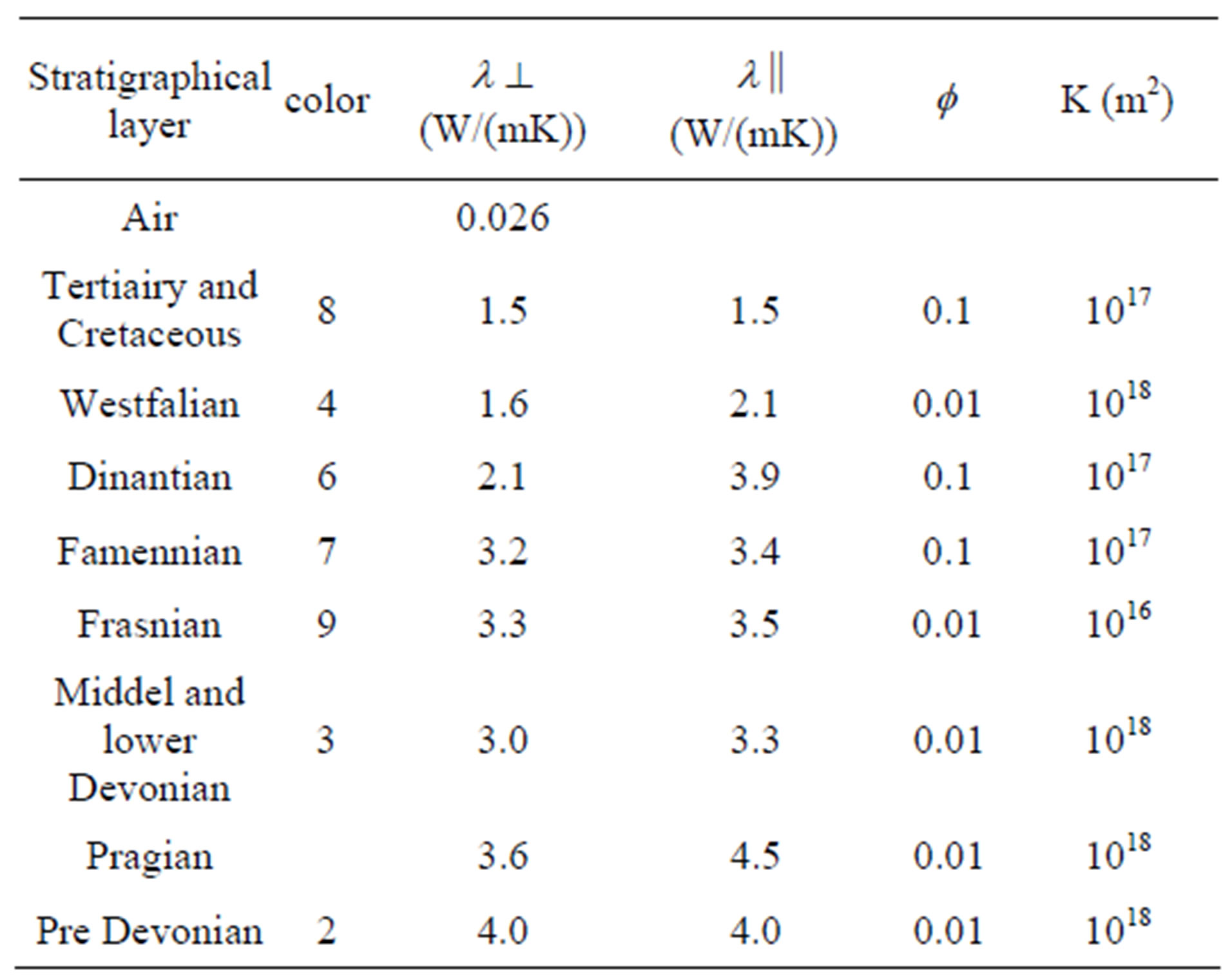
Table 4. Average thermal conductivity values  and
and  as well as porosity
  and permeability k derived from measured data or published lithology values and lithology volume percentages of rocks for each layer.
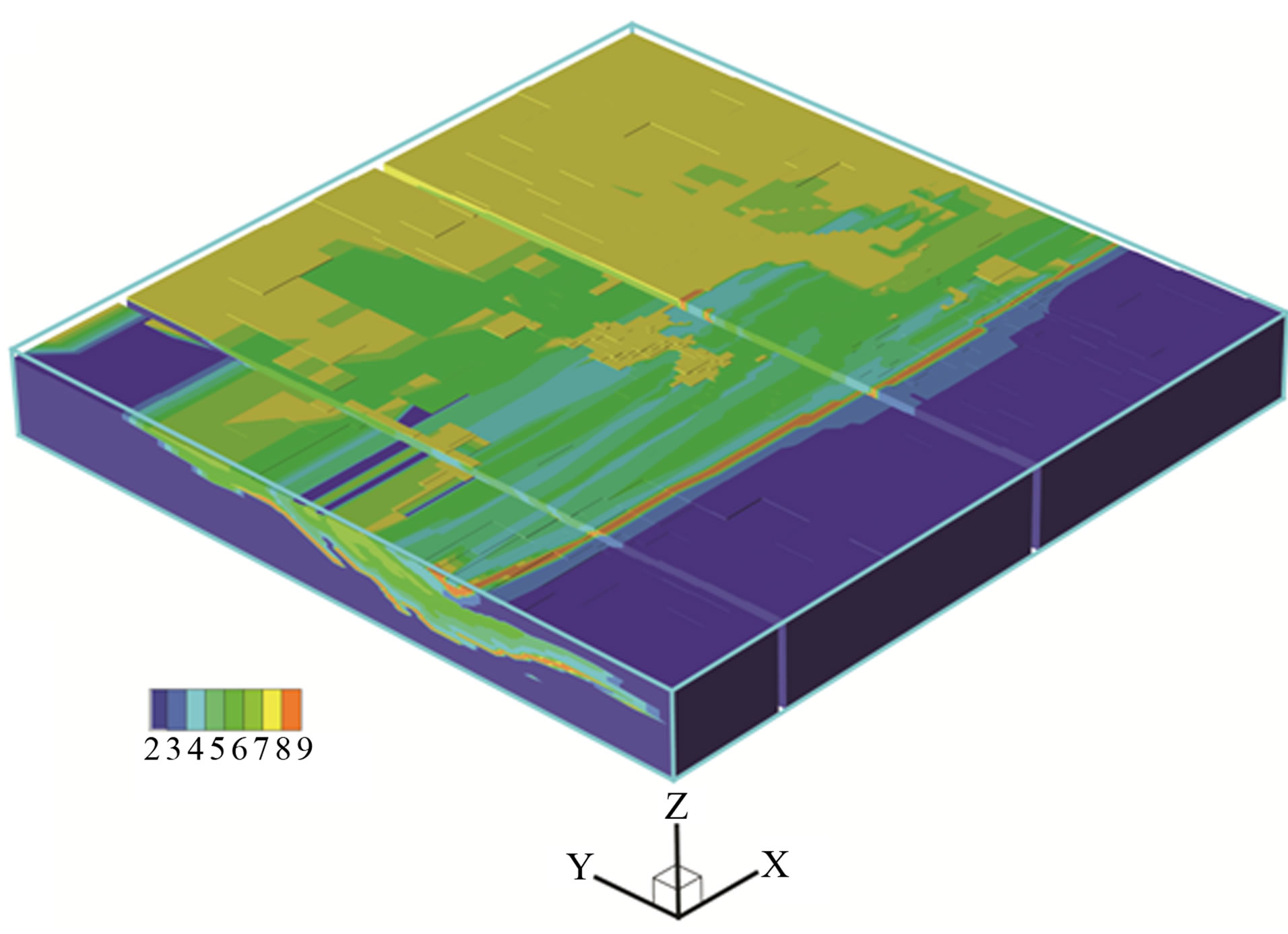
Figure 20. Stratigraphical 3D model with different stratigraphical units, with associated properties listed in Table 4.
surface elevation is implemented, using the Shuttle Radar Topography Mission-SRTM data 1 (see Figure 21) [39].
5.2. 3D Model Parameters
Orienting the 3D-grid of the numerical model for heat and fluid flow parallel to the main faults and along the subcrobs of the stratigraphical units, makes the creation of the model easier and more accurate.
To determine the percentage of different rocks in each stratigraphical unit, data from deep boreholes in the area have been used with the same stratigraphy.
Petrophysical properties are measured and inferred by use of cores, literature and logs. Thermal conductivity is based on measurements on cores performed at the University of Leuven (B) [33,40] and RWTH Aachen University (G) [41,42]. The mean properties for lithologies are translated into harmonic or geometric mean properties for each stratigraphy by use of weighting according to the percentage.
The heat production was derived from the specific gamma log and from the velocity log but is neglected in the model, because of the low value (<3 µW/m3) see [41,42]. Permeabilities are inferred from general values published in lit erature. Notice the very low porosity and permeability in the layers. Fluid flow is depending on fracture permeability rather than on primary rock porosity. Little is known about permeability at depth. As described in [41,42], permeability from the RWTH-1 Borehole is less than 10 - 15. In literature nothing is mentioned about fault permeability so when mentioned during modeling. some layers and fault zones are assigned a higher permeability and different scenario’s have been simulated.
The thermal conductivities of different lithologies were measured in similar stratigraphical units [33,43] yielding the average thermal conductivities listed in Table 5.
We derived from each stratigraphical laye, the percentages % of different rocktypes thickness’s with respect to the total thickness (see Figure 22). This is done with the use of different borehole logs and core measurements.
The average anisotropic values of thermal conductivity for each stratigraphical layer can now be determined from the arithmetic mean
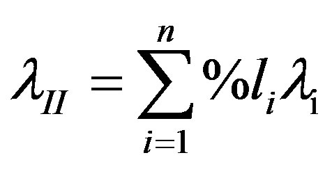 (9)
(9)
in case of a horizontal heat flux parallel to the layering, and from the harmonic mean
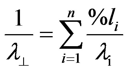 (10)
(10)
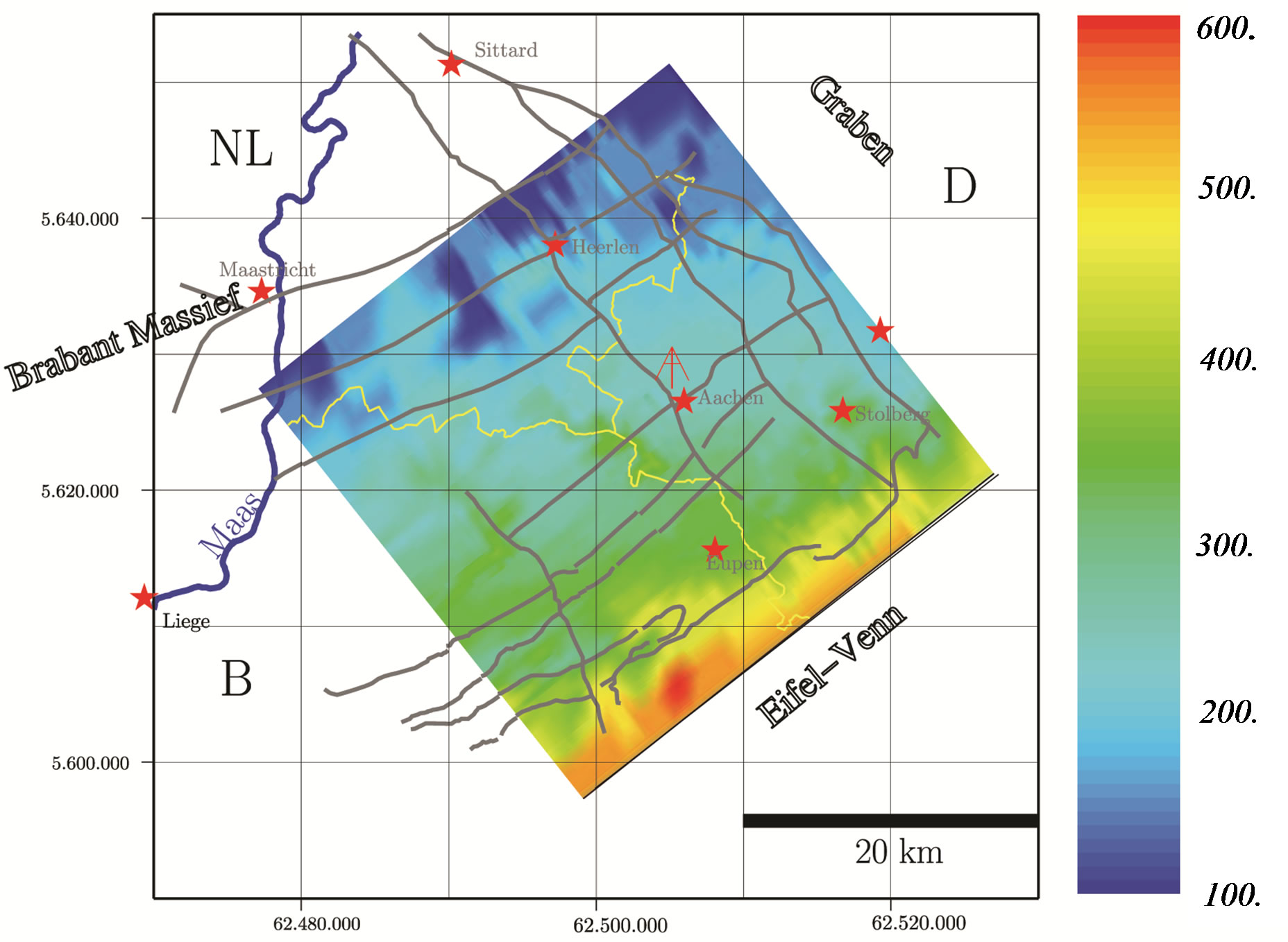
Figure 21. The elevation map in (m) used as boundary condition in the 3D model and the 2D cross sections.
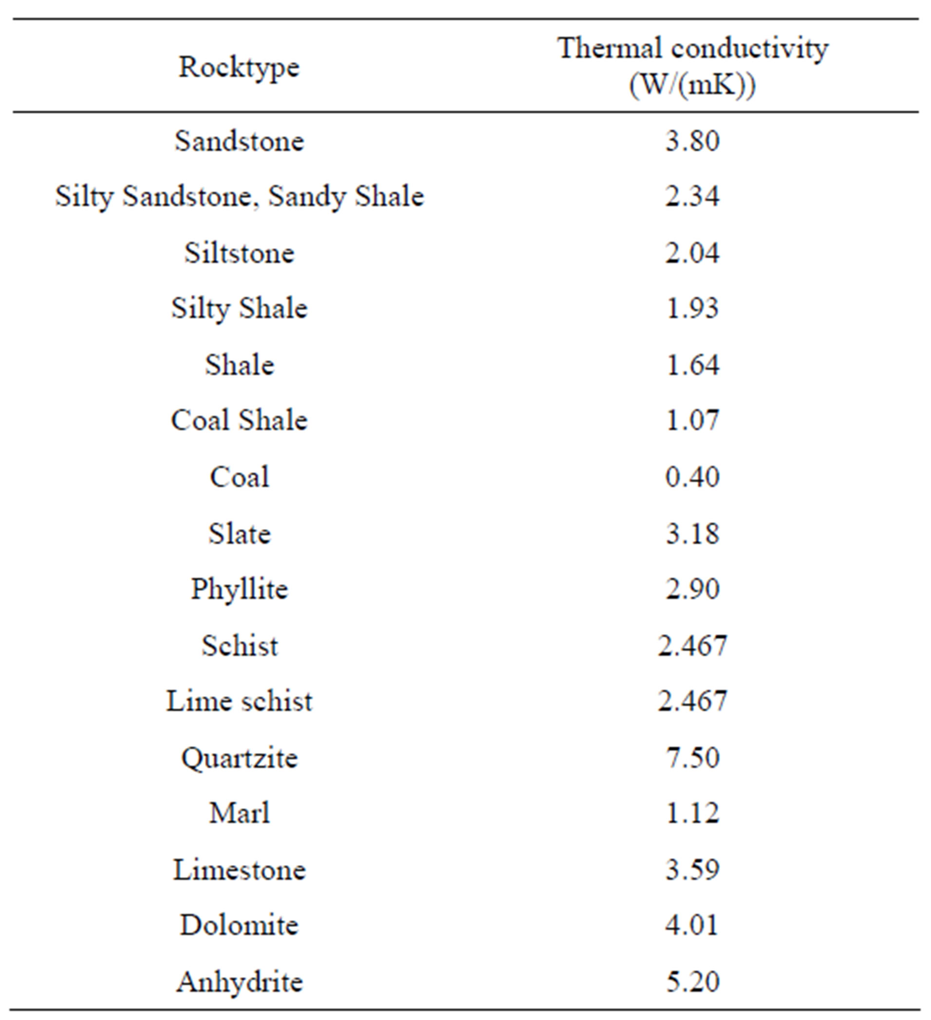
Table 5. Thermal conductivities of the different Rocktypes [33,43].
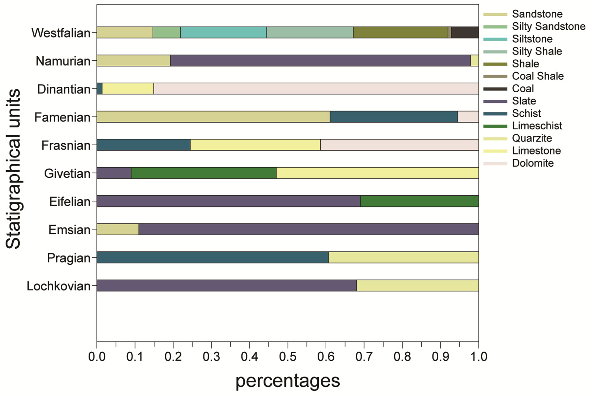
Figure 22. Stratigraphical layers with their percentage of lithographies.
in case of a vertical heat flux perpendicular to the layering. Table 4 lists the averages of measured thermal conductivities of each stratigraphical layer. Note the low thermal conductivities of the Westfalian. The low thermal conductivities from the Cretaceous and Tertiary are based on literature data of limestone and high porosity sediments.
The 3D model is 40 km by 40 km large and 5 km deep, with a uniform basement down to a depth of 30 km. The reason for including the basement is to avoid a boundary condition at a depth of 5 km. Temperature at the surface of the model is fixed at 10˚C, at the bottom of the model, in 30 km depth, at 750˚C. There is no heat flow across the lateral boundaries.
5.3. 3D Model Results
5.3.1. Effect of Differences in Thermal Conductivity
In the 40˚C iso-surface in the left part of Figure 23 coal bearing layers are indicated by low specific heat flow (0.06 mW/m2). At the borders of the low conductiveity layers, there is a lateral heat flow corresponding to a lateral variation in temperature gradient. This effect becomes smaller with distance from the boundary of the coal layers. A similar effect can be seen underneath a limestone hill in the center of the 15˚C iso-surface in the right part of Figure 23.
5.3.2. Effect of Deep Convective Water Flow on Heat Flow
Figure 24 shows the influence of deep water flow on specific heat flow. The variation in specific heat flow is directly related to the hydraulic conductivity of the layer with deep water circulation.
6. ACKNOWLEDGEMENTS
We would particularly like to thank Prof. Van den Berghe, of the University of Leuven for delivering their measurements of thermal conduc-
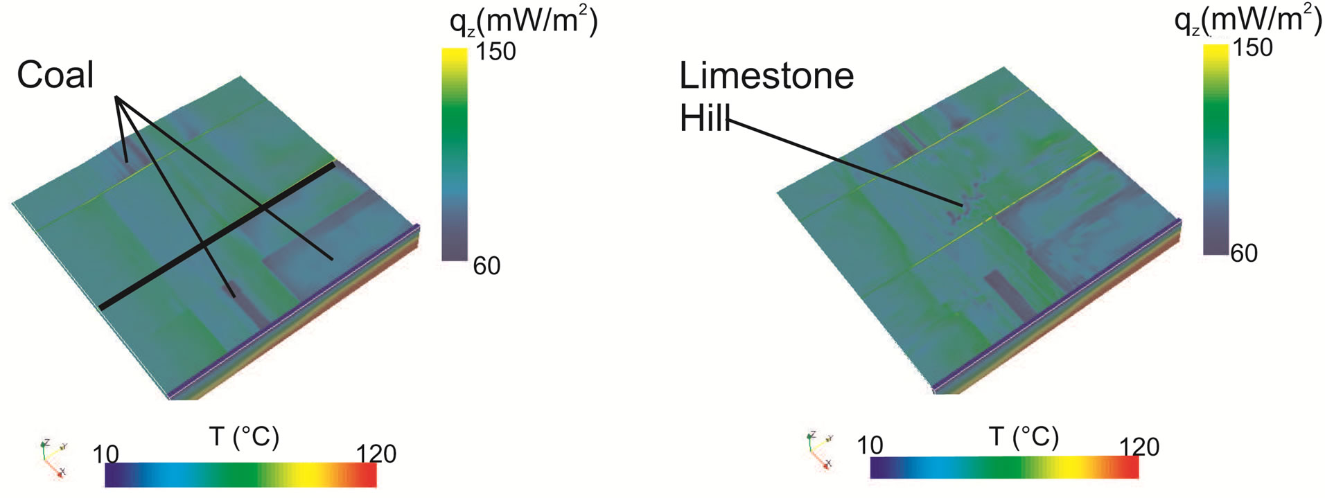
Figure 23. Left figure: In the 40˚C iso-surface coal bearing layers are indicated by low spec. heat flow (0.06 mW/m2). At the borders of the low conductivity layers, there is a lateral heat flow corresponding to a lateral variation in temperature gradient. This effect becomes smaller with distance from the boundary of the coal layers. Righ figure: Similar effect can be seen underneath a limestone hill in the middle of the 15˚C iso-surface.
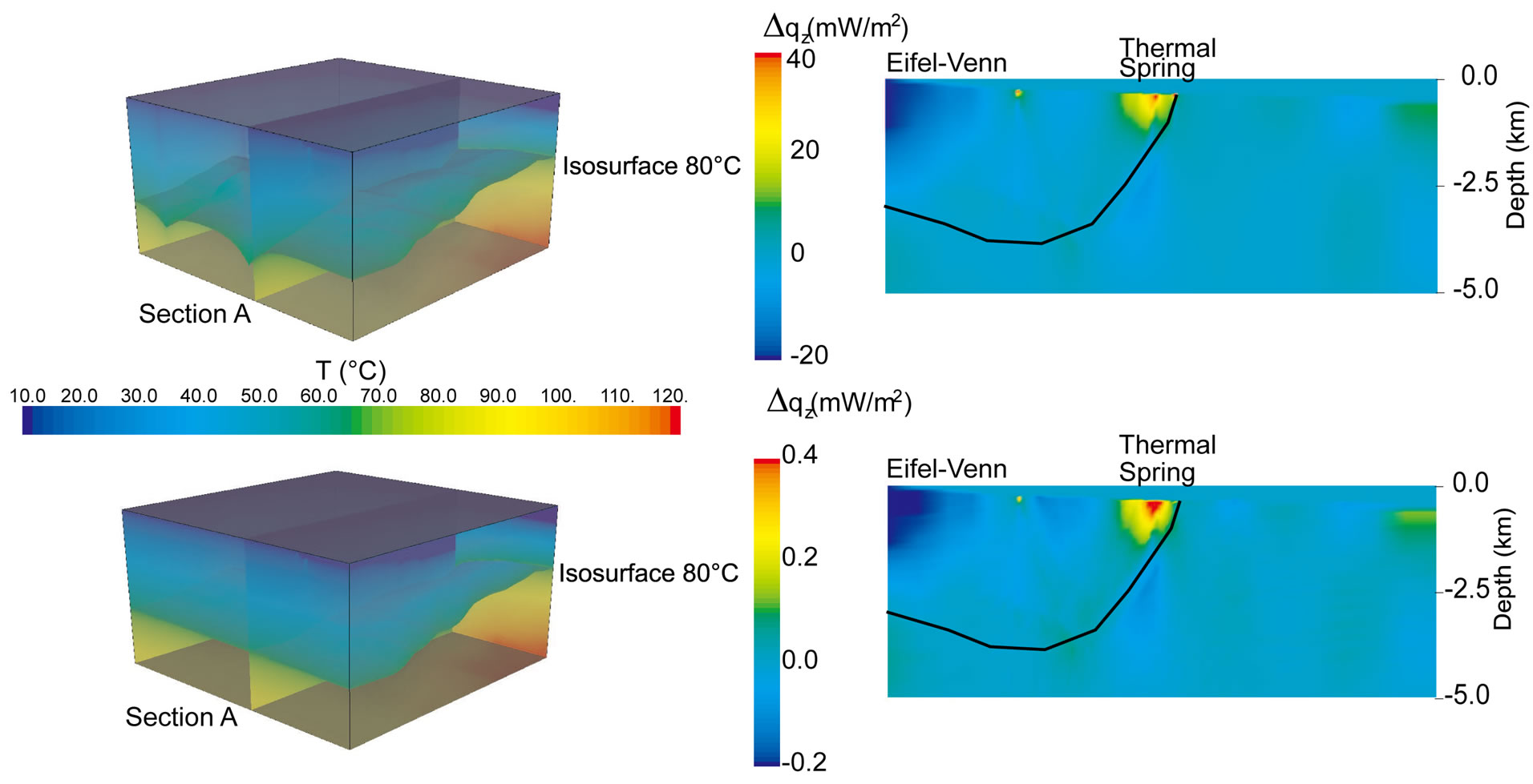
Figure 24. 3D temperature model with a) a hydraulic conductivity of 10 - 14 m2 and b) a hydraulic conductivity of 10 - 16 m2; Section A shows the heat flux variations due to the deep water flow and the geothermal springs in both cases.
tivities on cores of the Belgium deep boreholes and thank the Geological Surveys of the Netherlands, Belgium and Nordrhein-Westfalen for their great help for delivering core material, logs, maps and reports.
REFERENCES
- Ziegler, P. and Dèzes, P. (2005) Crustal evolution of western and central Europe. Memoir of the Geological Society, London.
- Walter, R. (2007) Geologie von mitteleuropa. Verslagbuchhandlung, Stuttgart.
- Van Tongeren, P. (2005) De vlaamse voerstreek: Een geologische analyse van het laat palaezoicum van deze regio en het direct aangrenzend gebied. Tech/Rep.
- Dewaele, S. and Muchez, P. (2004) Alteration, mineralisation and fluid flow. Geologica Belgica, 7, 55-69.
- Bless, M. and Bouckaert, J. (1988) Suggestions for a deep seismic investigation north of the variscan mobile belt in the se netherlands. Annales de la Societe geologique de Belgique, 111, 229-241.
- Hollmann, E. (1997) Der variszische vorlandsu¨berschiebungsgu¨rtel der Ostbelgischen Ardennen. Ph.D. Thesis, RWTH Aachen University, Aachen, Germany.
- Bless, M., Boukaert, J., and Paproth, E. (1980) Environmental aspects of some pre-Permian deposits in NW Europe. Mededelingen Rijks Geologische Dienst, 32-1, 3-13.
- Van Adrichem Boogaert, H. (1999) Toelichting bij kaartblad XV sittard maastricht. NITG-TNO Geological Survey, Utrecht.
- Arnold, J.W.S.H. and Schott, B. (2001) Continental collision and the dynamic and thermal evolution of the variscan orogenic crustal root—Numerical models. Journal of Geodynamics, 31, 273-291. doi:10.1016/S0264-3707(00)00023-5
- Von Winterfeld, C. (1994) Variszische Deckentek-tonik und devonische Beckengeometrie der Nordeifel—Ein quantitatives Modell (Profilbilanzierung und Strainanalyse im Linksrhenischen Schiefergebirge). Ph.D. Thesis, RWTH-Aachen University, Aachen.
- Lünenschloss, B., Bayer, U., and Muchez, P. (1997) Coalification anomalies induced by fluid flow at the variscan thrust front: a numerical model of the paleotemperature field. Geologie en Mijnbouw, 76, 271-275.
- Keyser, M., Ritter, J. and Jordan, M. (2002) 3D shearwave velocity structure of the Eifel plume, Germany. Earth and Planetary Science Letters, 203, 59-82. doi:10.1016/S0012-821X(02)00861-0
- Knapp, G., Gliese, J. and Hager, H. (1980) Geologische karte der nordlichen eifel 1:100000. Geologischen Landesamt Nordrhein-Westfalen, Krefeld.
- Bless, M., et al. (1980) Tiefenlage der Oberfla¨che des namurs. In: Mededelingen Rijks Geologische Dienst, 17- 32.
- Wrede, V. and Zeller, M. (1987) Geologische karte der aachener steinkohlenlagersta¨tte, dargestellt an der karbonoberflache 1:25000. Geologischen Landesamt Nordrhein-Westfalen, Krefeld.
- Bless, M., et al. (1980) Tiefenlage der oberflächedes Prä- Perms. Mededelingen Rijks Geologische Dienst, 17-32.
- Sauvage, C., Vanneste, C., Bertola, C., Dubois, D., Laloux, M., Willame, V. and Engels, P. (2005) Carte ge’ologique de Wallonie; la Direction Ge’ne’rale des Ressources Naturelles et de l’Environnement—Ministe`re de la Region Wallonne, Belgique. http://carto1.wallonie.be/geologie/viewer.htm
- Bosch, P., Kisters, P. and Felder, W. (1995) Geologische kaart van Zuid-Limburg en omgeving; Paleozocum 1: 50000 (geological map of Zuid-Limburg en surroundings). Rijks Geologische Dienst, Heerlen.
- Group, D. (1990) Results of deep-seismic reflection investigations in the rhenish massif. Tectonophysics, 173, 507-515.
- Group, D. (1991) Results of the dekorp 1 (belcorp-dekorp) deep seismic reflection studies in the western part of the rhenish massif. Geophysics Journal International, 106, 203-227.
- Leibecker, J. (2000) Elektromagnetische arraymes-sungen im rheinischen schiefergebirge: Modelle der elektrischen leitfahigkeit der erdkruste und des oberen mantels mit verbindungen zum eifelvulkanismus. Ph.D. Thesis, George-August-University Guttingen, Göttingen.
- Ritter, J., Jordan, M., Christensen, U. and Achauer, U. (2001) A mantle plume below the Eifel volcanic fields, Germany. Earth Planet Science Letters, 186, 7-14. doi:10.1016/S0012-821X(01)00226-6
- Granet, M., Wilson, M. and Achauer, U. (1995) Imaging a mantle plume beneath the French Massif Central. Earth Planet Science Letters, 136, 281-296. doi:10.1016/0012-821X(95)00174-B
- Anonymous (1976) Bouguer anomaly of belgium and surroundings. Observatoire Royal de Belgique.
- Wilson, J. (1966) Did the Atlantic close and then re-open? Nature, 211, 676-681. doi:10.1038/211676a0
- Kusznir, N. and Karner, G. (2007) Continental lithospheric thinning and responce to upwelling divergent mantle flow: Application to the Woodlark, Newfound-land and Iberia margins. Geological Society of London, London.
- Barker, C. and Pawlewicz, M. (1986) The correlation of vitrinite reflectance with maximum temperature in humic organic matter. In: Buntebarth, G. and Stegena, L., Eds., Lecture Notes in Earth Sciences, Paleothermics, Springer-Verlag, Berlin, 79-93.
- Pommerening, J. (1992) Hydrogeologie, hydrogeochemie und genese der aachener thermalquellen. Ph.D. Thesis, RWTH Aachen University, Aachen.
- Truesdell, A. (1976) Summery of section III: Geochemical techniques in exploration. Proceedings 2nd U.N. Symposium on the Development and Use of Geothermal Resources, US Government Printing Office, Washington.
- Gupta, H. (1980) Geothermal resources: An energy alternative of Developments in economic geology. Elsevier Scientific Publishing Company.
- Driesen, J. (1963) Mijnwater oranje nassau mijnen. Geologische Dienst O. N. Mijnen.
- Dèzes, P., Schmid, S. and Ziegler, P. (2004) Evolution of the European Cenozoic rift system: Interaction of the alpine and pyrenean orogens with their foreland lithosphere. Tectonophysics, 389, 1-33. doi:10.1016/j.tecto.2004.06.011
- Verkeyn, M. (1995) Bepaling van de Warme-stroomdichtheid in België-een verkenning naar de mogelijkheden en de beperkingen (Detemination of the Specific Heat Flow in Belgium with possibilties and limitations). Master’s Thesis, Kath University Leuven Belgium, Leuven.
- Rybach, L. (1979) The relationship between seismic velocity and radioactive heat production in crustal rocks; an exponential law. Pure and Applied Geophysics, 117, 75- 82. doi:10.1007/BF00879735
- Carslaw, H. and Jeager, J. (1946) Conduction of heat in solids. Oxford University Press, Oxford.
- Turcotte, D. and Schubert, G. (2002) Geodynamics. Cambridge University Press, Cambridge. doi:10.1017/CBO9780511807442
- Clauser, C. (2003) Numerical simulation of reactive flow in hot aquifers. Springer-Verlag, Berlin.
- Clauser, C. (1984) A climatic correction on temperature gradients using surface-temperature series of various periods. Tectonophysics, 103, 33-46.
- Anonymous (2005) Shuttle radar topography mission SRTM data.
- Denhaene, T. (1997) Bepaling van de warmte-stroom uit boorgaten in Belgie. Master’s Thesis, Kath. University Leuven, Leuven.
- Dijkshoorn, L. and Pechnig, R. (2007) Physical properties in the carboniferous and devonian rocks drilled in the rwth-1. Jahrestagung der Deutschen Geophysikalischen Gesellschaft, Aachen.
- Dijkshoorn, L. (2012) The earth as energy stock—Natural and enhanced behavior of thermal resistances, heat storage capacity and heat flow in the earth and their relevance to the geothermal power of a deep coaxial borehole heat exchangerin the Eifel-Maas region. Ph.D. Thesis, RWTH Aachen University, Aachen.
- Speer, S. (2005) Design calculations for optimising of a deep borehole heat-exchanger. Master’s Thesis, RWTH Aachen University, Aachen.