Engineering
Vol.10 No.10(2018), Article ID:87939,26 pages
10.4236/eng.2018.1010051
The Implementation and Lateral Control Optimization of a UAV Based on Phase Lead Compensator and Signal Constraint Controller
Adil Loya1, Muhammad Duraid1, Kamran Maqsood2, Rehan Rasheed Khan3
1Department of Mechatronics Engineering, PAF Karachi Institute of Economics and Technology, Karachi, Pakistan
2School of Engineering and Informatics, Sussex University, Brighton, UK
3Department of Avionics Engineering, PAF Karachi Institute of Economics and Technology, Karachi, Pakistan

Copyright © 2018 by authors and Scientific Research Publishing Inc.
This work is licensed under the Creative Commons Attribution International License (CC BY 4.0).
http://creativecommons.org/licenses/by/4.0/


Received: September 5, 2018; Accepted: October 20, 2018; Published: October 23, 2018
ABSTRACT
Unmanned Aero Vehicles (UAV) has become a useful entity for quite a good number of industries and facilities. It is an agile, cost effective and reliable solution for communication, defense, security, delivery, surveillance and surveying etc. However, their reliability is dependent on the resilient and stabilizes performance based on control systems embedded behind the body. Therefore, the UAV is majorly dependent upon controller design and the requirement of particular performance parameters. Nevertheless, in modern technologies there is always a room for improvement. In the similar manner a UAV lateral control system was implemented and researched in this study, which has been optimized using Proportional, Integral and Derivative (PID) controller, phase lead compensator and signal constraint controller. The significance of this study is the optimization of the existing UAV controller plant for improving lateral performance and stability. With this UAV community will benefit from designing robust controls using the optimized method utilized in this paper and moreover this will provide sophisticated control to operate in unpredictable environments. It is observed that results obtained for optimized lateral control dynamics using phase lead compensator (PLC) are efficacious than the simple PID feedback gains. However, for optimizing unwanted signals of lateral velocity, yaw rate, and yaw angle modes, PLC were integrated with PID to achieve dynamical stability.
Keywords:
Lateral Control, Simulink, PID Signal Constraining, Phase Lead Compensators, Unmanned Aero Vehicle

1. Introduction
In this new era, Unmanned Aerial Vehicle (UAV) is used for many applications. With different applications of UAV’s, mission characteristics also changes with specific requirements. However, with these maximum numbers of applications there are many difficulties that happen in real time scenario. In the practical atmosphere; it is very necessary that UAV must be fully controlled and impulsive. Controllability and response is totally dependent upon the controller or controlling techniques that are being used [1] . Moreover, UAV controllability depends on the nonlinear factors i.e. aerodynamics variables. UAV performance characteristics are determined by its flight controller mechanism, which controls the dynamics of a UAV [2] . Likewise, there has been lots of research on flight control optimization using different control techniques. To cater above, different control techniques have already been designed and implemented in UAVs flight control systems such as adaptive control, robust control, predictive control, optimal control, and intelligent control [3] [4] . Moreover, it is known from studies and literature that Proportional, Integral and Derivative control approach is not new, however, due to its easiness for implementation in hardware and software, maintenance is less so it is preferable over other control techniques [5] . But, there is less adaptability for PID, as they are not able to produce good performance output when tested in a real-world UAV [6] [7] . The conventional approach for optimizing PID performance is to use PID with gain scheduling [8] . The swapping between different controllers during flight is not always smooth, therefore it is important to design a single flight controller for a complete flight envelope [9] [10] . On the other hand, PID control algorithms are more attractive in terms of practically designing optimized controllers for UAV’s. This is not only due to their easy modeling and simple implantation, but as well as their safe and stable performance. Moreover, in PID controller, tuning is a critical task to achieve optimal values for PID gain parameters [11] . Many methods are found to set the parameters of PID controller in the literature, i.e. internal model-based design control (IMC), the Ziegler-Nichols method and loop shaping method. All of these methods are founded on some basic characteristics of plant models. PID controller gain parameters are settled down according to certain properties and algorithms that are basis for particular plant [12] . The tuning of PID gains is still worth putting effort and for which various techniques for fine tuning PID gains are already available [13] . The Ziegler-Nichols is a most well-known technique in the field of PID tuning. It is easily utilized for fine tuning the PID but its performance lacks in nonlinear systems [14] . Moreover, optimal control technique is also utilized for PID gain scheduling. Moreover, considerable research has been carried out in designing algorithms for UAV using modern control theory. While in the navigation and control domain large number of onboard control algorithms has been developed. Most of the times, some non-linear techniques have been used to optimize model with high control response. In spite of their revolutionary success, few of them are used and implemented. Likewise, Sheibani investigated that by applying PID controllers on lateral and longitudinal stability optimizes the performance of the aircraft dynamics. PID controller efficaciously improved the settling time and over shoot harmonics were undermined, this demonstrates that significant amount of controllability has been achieved [15] .
Controlling UAVs has become a hot topic for last couple of years. So, the term controllability is the property that determines the performance, that how much a system is reliable and stable for different input parameters. Actual working of PID is to shift poles of the system from right half plane to left half plane in root locus plot using PID gain scheduling, by doing so system becomes stable. Moreover, Muluken Regas in his research used PID with neural network controller giving insight into optimization of PID using neural networks. They compared UAV’s pitch altitude control parameters developed by each controlling techniques. Thus, they concluded that for hardware implementation of any UAV model with smooth alteration to achieve better maneuverability, PID is a prime candidate for the designing of optimized controller [16] .
Keeping in mind the researches related with PID optimization and checking out the literature; it is pretty much applicable that there is still room for improvement. Hence in this research efforts have been plugged to optimize PID using signal constraining and Phase Lead Compensator (PLC).
Nevertheless, in some cases of controlling lateral mode PID controller is not feasible enough to give steady state response, therefore, a good practice in this case is to implement a phase lead compensator. The PLCs are generally used for improving the transient response of a dynamic system. This controller adds up positive contribution in the sum of angles in the angle measurement. It helps in moving the close loop poles towards the negative half of the s-plane, due to which stability and speed of the system response is optimized. This technique is proven to be fruitful in one of the studies investigated for pitch and altitude control by Ahsan et al. [17] . They investigated that by using a PLC, transient response characteristics were improved as compared to PID controller. However, the PLC takes longer rise time for his case, but offers negligible overshoots.
2. Plant Description
An initial design for this proposed model of UAV was created using XFLR5, a freeware software used for designing and modelling flight dynamics of UAVs. XFLR5 Plane designing module lets one to easily design, as well as, visualize the input variables while changing different design parameters of the aircraft body [18] . Moreover, aerodynamic stability parameters were obtained from the same software, which were used to form a mathematical model for the UAV’s transfer function plant design. Furthermore, transforming system characteristics matrix and state space model is converted to transfer function which helps in further analyzing model stability. This obtained mathematical model is used to formulate the longitudinal and lateral transfer functions. Mathematical modeling of plant is necessary for the practical design of an UAV. In addition to this, the mathematical model is a fundamental plant for designing of an open loop system. Nevertheless, plant designing further requires a feedback response, for which a closed loop system is integrated using PID control technique. The PID controller was implemented to stabilize the response of the control surfaces by decreasing the overshoot and optimizing the settling time to meet the monotonic decay.
The longitudinal equations for the plant are derived by applying laws of newton for the motion of a rigid body under the effect of constant external forces and moments summation to the angular acceleration. These are the following assumptions taken for simulating proposed model equations [19] .
Assumptions taken; the geometrical shape parameters are jotted in Table 1, moreover some of the configuration, stability and control parameters were obtained from author’s previous study [18] . Stability analysis of UAV model requires, aerodynamic analysis of complete UAV plant to measure its different stability coefficients. The proposed model was analyzed using Vortex lattice method (VLM), while coefficient of X-Center of Gravity and Z-Center of Gravity was set at 0.09 m and 0.003 m respectively. Moreover, proposed plant was experienced with 35 m/s velocity and density for the physical attributes were settled at 1.225 Kg/m3, meanwhile the viscosity level was 1.461e-5 m2/s and Dirichlet boundary were set for analysis.
1) The Earth is non-rotating.
2) Unmanned aero vehicle is supposed to be a constant mass rigid body.
3. Working
MATLAB/Simulink simulation is used to incorporate the proposed model, which was achieved by designing of UAV model on XFLR5. Stability and control derivatives were also obtained and calculated through XFLR5. These derivatives and parameters for transfer functions were plugged in the MATLAB prompt to generate the longitudinal and lateral matrix. The parameters used for designing the transfer function are given in Table 1; this enabled us to design the transfer function from its state space model. Moreover, the initial control outputs determined using open loop system approach gave unstable response, obviously, system requires a feed-back response inherited with a certain controller to stabilize its response. While in this proposed study, PID was implemented for system response refinement and phase lead compensators were used for optimizing unstable dynamics of certain inputs that were not easily controlled by PID. Likewise, Rudder and Aileron parameters obtained through PID controller demonstrated stable characteristics, but 2 parameters from the both groups were further stabilized through compensating gain technique. A schematic design shows the workflow of this research in Figure 1.
The lateral stability derivative parameters for design of transfer function were obtained from XFLR5 as shown in Table 2.
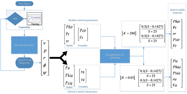
Figure 1. Schematic of the workflow that has been performed in this research.

Table 1. UAV design specifications [7] .
Table 2. Lateral stability parameters.
(1)
(2)
By using Equations (1) and (2) and Table 1 data, state space model for the lateral dynamics was established. This lateral plant was then divided into five lateral variables that x = [v p r phi psi]; where x is the output variable that consist of v which is “lateral velocity component”, p is “roll rate component”, r is “yaw rate component”, phi is “roll angle component”. Multiple Input and Multiple Output (MIMO) system transfer function equations were designed out of these multi variable outputs (these equations are shown from Equations (3) to (12), where input variables controlling these equations were two i.e. one is for aileron input dependent represented by “Yda” and other one is rudder input dependent “Ydr”. Transfer functions acquired for state space model are given from Equations (3)-(12) in Table 3 and Table 4.
3.1. Plant Description When in Loop with PID
We can describe PID controller with following continuous S domain transfer function.
(13)
where , and are the proportional gain, integration and derivative coefficients. These are the feed-back gains used to stable the response of plant. In cases critical load disturbance and set-point tracking are desirables the set-point weighting technique is used for the optimization. There is always a steady state error presented in any practical system because if system will be designed it’s essential to have some stable region where output of that system responds linearly as input changes. Therefore, considering only proportional control gives us tendency with increase gain and as well oscillations. As compared to proportional
Table 3. UAV lateral dynamic transfer functions with respect to aileron input.
Table 4. UAV lateral dynamic transfer functions with respect to rudder input.
control, integral controller is always used to decrease the error after this implementation, tendency towards oscillations increases with the decrease in integral time. Moreover, integral coefficient minimizes the steady state error. However, derivative term is used to decrease the damping effect on closed loop response, initially damping increases with small increase of derivative time, however, with large derivative damping becomes minimal. In this proposed research root locus based PID controller is implemented for the lateral control, using lateral sub-model of a UAV.
3.2. Plant Description When in Loop with Signal Constraining PID
Signal Constraint predictive control (SCPC) is a technique used in industrial level to control unpredicted system parameters [20] . Earlier signal constraint control was only used in dynamically slow processes due to this compensation required for optimization took too much time. With the advancement in automatic computational algorithms the use of SCPC is now more feasible and reliable. Fast computing also made this process efficient and safer for UAV applications. Therefore, due to fast computing invention, it is now possible to use SCPC in dynamically fast process like civil air-vehicles. In this proposed model objective of this computational signal constraining is to attain future predictions for optimized control of different parameters sequence. Hence, predicted outputs could be used to drive UAV with more optimized and stable way. Moreover, to predict future process outputs for the control variables, this topology explicitly uses mathematical model [20] . A signal constrained optimization technique general output overview is shown in Figure 2.
3.3. Plant Description When in Loop with Lead Compensator
General equation for frequency domain description for phase lead compensator is given by Equation (4) [17] ;
(14)
where z0 and p0 are the zero and pole of the compensator respectively and Kc is the controller gain. Moreover, for lead compensator zeros should be less than the number of poles i.e. z < p. In addition to phase lead compensator for the lateral controller, a yaw angle washout filter in the feedback loop is applied to the lateral sub-model for increasing the system yaw damping mode. This loop is acting in phase lead compensation mode. The block diagram of the control loops of phase lead compensator introduced with lateral velocity and yaw rate are shown in Figure 3. Where Kc is a gain for compensation and for lateral case when rudder is being used as an input “Kc = 288”. The difference between desired yaw angle and current aircraft yaw angle is the error signal acting as the reference input for the yaw angle control loop. The gains of the phase lead compensator, as well as the positions of its zero and pole are varied to track the step input at the ailerons.

Figure 2. Signal constraint model.

Figure 3. Connection of lead compensators with lateral plant for compensating output signal i.e. (a) lateral velocity compensation and (b) yaw rate compensation.
(15)
Designing a PLC is carried out using root locus technique. The lateral velocity and yawing angle with respect to aileron input for stable response is controlled with PLC, which is sketched in methodology section.
4. Results and Discussion
The optimization of any new unmanned vehicle for stability and control correctness is necessary. As per our design is concerned it was necessary to smoothen the lateral flight dynamics of the UAV while in flight for which, PID and PID signal constraining was used. In this section results and discussion has been presented for controlling rudder and aileron dynamics. First section is lateral control when rudder is selected as an input and second section is lateral control when aileron is selected as an input.
4.1. Lateral Control When Rudder Is Selected as an Input
This section holds results and discussion of lateral mode control using rudder as an input variable. In this section five major output variables of lateral dynamics are controlled using rudder. Those five output variables are [v p r phi psi].
4.1.1. Lateral Roll Rate Dynamics Dependent on Rudder Input (PR)
Lateral mode gain setting for roll rate dynamics dependent on rudder input are displayed in Table 5.
Figure 4 represents the stabilization of the rudder input on the roll rate. This can be observed in the closed loop response Figure 4(c) and its root locus are within the proximity of negative s-plane. Moreover, the rudder has little or less effect on the rolling moment of the aircraft. Therefore, it gets stabilized quickly from a disturbed mode.
4.1.2. Lateral Roll Angle Dynamics Dependent on Rudder Input (PHIR)
Lateral mode gain setting for roll angle dynamics dependent on rudder input are displayed in Table 6.
Table 5. UAV roll rate dynamics dependent on Rudder input (pr).
Table 6. UAV roll angle dynamics dependent on Rudder input (phir).

Figure 4. Root locus and step response of lateral roll rate dynamics dependent on Rudder input (a) open loop step response, (b) root locus of open loop system, (c) closed loop step response and (d) root locus of closed loop system.
Figure 5 represents the stabilization of the rudder input on the roll angle. This can be observed in the closed loop response Figure 5(c) and its root locus are within the proximity of negative s-plane. Moreover, the rudder has little or less effect on the rolling moment of the plane. Therefore it gets stabilized quickly from a disturbed mode. However, initially the response of the closed loop gain is taking time to settle down from disturbed oscillations to steady state. In terms of rolling motion induced due to roll angle, Dutch roll performance is present in the negative s-plane, however, near to the complex axis, demonstrating boundary level stability.
4.1.3. Lateral YAW Angle Dynamics Dependent on Rudder Input (PSIR)
Lateral mode gain setting for yaw angle dynamics dependent on rudder input are displayed in Table 7.
Figure 6 is representing unstable response after setting the closed loop gains for yaw angle with respect to rudder input. This is because the rudder has high influence on the yaw angle of the UAV. Therefore, it requires a compensator to overcome this divergence from the unstable zone. In addition to this, compensator was added as shown in Equation (16) to the feedback response of the controller to stabilize the yawing angle with respect to rudder input. This compensator helps in damping out the unwanted vibrations and oscillations involved in destabilizing of the control surface as shown in Figure 7(a) by the step response of the yaw angle dependent on rudder input. Moreover, the root locus is also in the negative half of the s-plane as shown in Figure 7(b).

Figure 5. Root locus and step response of lateral roll angle dynamics dependent on Rudder input (a) open loop step response, (b) root locus of open loop system, (c) closed loop step response and (d) root locus of closed loop system.

Figure 6. Root locus and step response of lateral yaw angle dynamics dependent on Rudder input (a) open loop step response, (b) root locus of open loop system, (c) closed loop step response and (d) root locus of closed loop system.
 (a) (b)
Figure 7. When a compensator is added to the psi angle with respect to rudder input; (a) step response (b) root locus.
Table 7. UAV YAW angle dynamics dependent on Rudder input (psir).
Added compensator:
(16)
with a K = 0.01.
4.1.4. Lateral Yaw Rate Dynamics Dependent on Rudder Input (RR)
Lateral mode gain setting for yaw rate dynamics dependent on rudder input are displayed in Table 8.
Figure 8 demonstrates stability in the yawing rate of the UAV after initializing the robust control gains. The stability is demonstrated for the spiral and roll modes, however, spiral mode is marginally stable as it is on the complex axis as shown in Figure 8(d).
4.1.5. Lateral Velocity Dynamics Dependent on Rudder Input (VR)
Lateral mode gain setting for lateral velocity dynamics dependent on rudder input are displayed in Table 9.
Figure 9 presents high rate of instability for sideslip velocity component when rudder input is used. However, balancing this requires a compensator to be placed, which damps out the response of sideslip entropy. Therefore, compensator was added in a lead/lag fashion with a gain as shown in Equation (17). By adding the compensator demonstrated marginable stability over the previous closed loop results without any compensator. This compensator helps in damping out the unwanted vibrations and oscillation involved in destabilizing of lateral velocity as shown in Figure 10(a) by the step response of the sideslip velocity dependent on rudder input. Moreover, the root locus plot in Figure 10(b) demonstrates the close loop poles are now in negative s-plane region than what was seen before without a compensator in Figure 9(d).
Table 8. UAV yaw rate dynamics dependent on Rudder input (rr).
Table 9. UAV velocity dynamics dependent on Rudder input (vr).

Figure 8. Root locus and step response of lateral yaw rate dynamics dependent on Rudder input (a) open loop step response, (b) root locus of open loop system, (c) closed loop step response and (d) root locus of closed loop system.

Figure 9. Root locus and step response of lateral velocity dynamics dependent on Rudder input (a) open loop step response, (b) root locus of open loop system, (c) closed loop step response and (d) root locus of closed loop system.
 (a)
(a) (b)
(b)
Figure 10. Root locus and step response of lateral velocity dynamics dependent on Rudder input (a) step response and (b) root locus.
Added Compensator:
(17)
with a K = 0.01.
4.2. Lateral Control When Aileron Is Selected as an Input
This section holds results and discussion of lateral mode control using aileron as an input variable. In this section five major output variables of lateral dynamics are controlled using aileron. Those five output variables are [v p r phi psi].
4.2.1. Lateral Roll Rate Dynamics Dependent on Aileron Input (PA)
Lateral mode gain setting for roll rate dynamics dependent on aileron input are displayed in Table 10.
The plot (c) in the Figure 11 shows poles in the negative region of the root locus plot. The modes that can be observed are related with Dutch roll motion of aircraft as the poles are standing on −7.72 ± 8.66 i. The value shows that Dutch roll performance of this aircraft while having input from aileron will give stable performance. Moreover, the rolling mode can create misleading movement in the aircraft motion which can cause undesired banking of the aircraft towards either of the x-axis ultimately making the aircraft to go in spiral mode, therefore, to tackle its stabilization with respect to roll-axis i.e. (x-axis) signal constrained PID were implemented to improve the stability response. In the meanwhile, the closed loop step response shows that the minimum settling time for roll rate on aileron input is less than one second.
4.2.2. Lateral Roll Angle Dynamics Dependent on Aileron Input (PHIA)
Lateral mode gain settings for roll angle dynamics dependent on aileron input are displayed in Table 11.

Figure 11. Root locus and step response of lateral roll rate dynamics dependent on aileron input (a) open loop step response, (b) root locus of open loop system, (c) closed loop step response and (d) root locus of closed loop system.
Table 10. UAV roll rate dynamics dependent on Rudder input (pa).
Table 11. UAV roll angle dynamics dependent on aileron input (phia).
From the close loop root locus plot of the Figure 12 part (d), some depictions on roll mode and Dutch roll stability can be witnessed. The roll angle stability performance using aileron input is found to control Dutch roll mode around −0.191 ± 2.43 which is in comparatively low stability to that of the roll rate input. Moreover, the roll mode performance is in highly stable region of root locus plot when aileron inputs are considered. Aircraft stability about longitudinal axis is also dependent on the roll angle which is an integral response of the roll rate, nevertheless, in Figure 12(c), settling time of closed loop response is stable, demonstrating the banking of aircraft at any particular angle using aileron will give stable response.
4.2.3. Lateral YAW Angle Dynamics Dependent on Aileron Input (PSIA)
Lateral mode gain setting for yaw angle dynamics dependent on aileron input are displayed in Table 12.
The closed loop response of rudder deflection variation due to aileron input in Figure 13(d) demonstrates Dutch roll mode in stable region as depicted earlier before with roll angle and roll rate. This shows that the UAV performance from the control perspective will be highly controllable. Moreover, the roll mode pole in Figure 13(d) is also in controllable region of root locus plot with a stable closed loop step response observed from Figure 13(c). Initially the response overshoots oscillations up to 20 seconds shows adverse yaw effect over the aircraft motion. But the close loop model parameters are deviating the adverse oscillations to a monotonic decay.
4.2.4. Lateral Yaw Rate Dynamics Dependent on Aileron Input (RA)
The poles on root locus graph of yaw rate dependent on aileron input demonstrates Dutch roll performance of the UAV, moreover, similar kind of response was found by Ihnseok Rhee et al. [21] while designing the auto pilot for a targeting drone. They used a Dutch roll filter to overcome this instability in drone dynamics. Lateral mode gain setting for yaw rate dynamics dependent on aileron input are displayed in Table 13.
Table 12. UAV YAW angle dynamics dependent on aileron input (psia).
Table 13. UAV YAW rate dynamics dependent on aileron input (ra).

Figure 12. Root locus and step response of lateral roll angle dynamics dependent on aileron input (a) open loop step response, (b) root locus of open loop system, (c) closed loop step response and (d) root locus of closed loop system.

Figure 13. Root locus and step response of lateral yaw angle dynamics dependent on aileron input (a) open loop step response, (b) root locus of open loop system, (c) closed loop step response and (d) root locus of closed loop system.
From Figure 14(c) it is depicted that the closed loop response is not settling, however, to further control compensator gains will be required for signal compensation. Moreover, closed loop root locus show that gains are in the right half of s-plane therefore, Dutch roll response is unstable. Reason behind this instability is because yaw rate is hard to stabilize while controlling with aileron. Nevertheless, spiral and roll mode poles are located in negative half plane showing the controllability of the UAV. However, in addition to this a compensator was used as a washout filter as shown in equation 18 to control the undesired response of the yaw angle due to aileron input. This compensator also acts as a yaw damper. Results of the yaw damper show that the response of the yaw angle is now in controllable region by which pilot has got enough room for response and to control the aircraft dynamics. Figure 15(b) shows yaw damping by adding washout filter demonstrating high controllability over the Dutch roll response, however, without compensator as shown in Figure 14(d), it is highly uncontrollable. Moreover, the step response after implementing compensator demonstrates stability and monotonic decaying of the response signal for a longer time period giving room to pilot over controlling of yaw moment. Due to the fact of practical implementation of maneuverability it is desired to have damped response with marginally instable spiral mode, so that pilot has room for maneuvering the aircraft easily. Therefore, using phase lead compensator apparently helps in achieving desired damped response by introducing certain zeroes and poles, where number of zeros is greater than the poles for PLC. Moreover, frequency, gain and phase margin are tweaked to achieve desired response. As compared to PID for the controlling step response of yaw rate with respect to aileron input compensator technique is more preferable as shown in Figure 15(a).
Added compensator:
(18)
with a gain Ka of 288.
4.2.5. Lateral Velocity Dynamics Dependent on Aileron Input (VA)
Lateral mode gain setting for lateral velocity dynamics dependent on aileron input are displayed in Table 14.
Figure 16 shows effect of aileron input on the sideslip velocity, it is depicted from above figures that using aileron, sideslip velocity cannot be controlled as it is dependent more on rudder rather than aileron. Moreover, the aileron effects are induced on the x-axis rather than z-axis. This enables smooth control of the rolling not for yawing motion. However, a compensator was added as shown by Equation (19) for controlling the sideslip velocity of the UAV and marginable control was achieved as shown by the Figure 17(b) root locus of the sideslip velocity with respect to aileron input. Moreover, the step response is also stable after adding a lead compensator to the lateral plant model. When we are using the PID controller, the response of the lateral velocity with respect to aileron input shows instability. Therefore, to stabilize the response of lateral velocity washout filter in a phase lead compensator arrangement has been inherited to overcome the instability. Moreover, in this case for better transient response phase lead compensator is more preferable due to its minimum rise time to desired lateral response as shown in Figure 17(a).
The compensator that was added to tackle the oscillation is shown in Equation (19); it is a lead compensator as the number of zeros are less than the number of poles.
Added compensator:
(19)
and also a gain with it K = 288.
Table 14. UAV velocity dynamics dependent on Rudder input (va).

Figure 14. Root locus and step response of lateral yaw rate dynamics dependent on aileron input (a) open loop step response, (b) root locus of open loop system, (c) closed loop step response and (d) root locus of closed loop system.
 (a)
(a) (b)
(b)
Figure 15. Washout filter applied to yaw angle with respect to aileron input; (a) step response and (b) root locus.

Figure 16. Root locus and step response lateral velocity dynamics dependent on aileron input (a) open loop step response, (b) root locus of open loop system, (c) closed loop step response and (d) root locus of closed loop system.
 (a)
(a) (b)
(b)
Figure 17. Washout filter applied to sideslip velocity with respect to aileron input; (a) step response and (b) root locus.
5. Conclusion
Current study has contributed with a great zeal on the topic of modelling of stable lateral UAV control dynamics using PID, PID Signal constraining and PLCs. It has been seen that the PID is capable of controlling different modes of the lateral dynamics with less overshoots and settling time. However, some numerical values were hard to analyze for which PID signal constraining was carried out, which enabled to get more precise estimations with considerable optimization in overshoots and settling times. Nevertheless, there were 4 transfer functions that were not easily controllable using either PID or PID signal constraining so PLCs were introduced. PLCs helped in optimizing step outs as well as stretched the poles in the negative half domain of S-plane. This enabled smooth and stable response from the unstable plants that involved; 1) lateral velocity dynamics on rudder input, 2) yaw angle dependent of rudder input, 3) lateral velocity dependent of aileron input, and 4) lateral yaw rate dependent on aileron input. Moreover, this research is currently limited to lateral control however, longitudinal control of UAV will be considered for future work with LQR/LQG and Sliding Mode (SM) controllers will be adopted for further smoothness of settling time and overshoots.
Acknowledgements
It is to acknowledge that there is no conflict of authors, as well as, we regards PAF Karachi Institute of Economics and Technology in support for this work.
Conflicts of Interest
The authors declare no conflicts of interest regarding the publication of this paper.
Cite this paper
Loya, A., Duraid, M., Maqsood, K. and Khan, R.R. (2018) The Implementation and Lateral Control Optimization of a UAV Based on Phase Lead Compensator and Signal Constraint Controller. Engineering, 10, 704-729. https://doi.org/10.4236/eng.2018.1010051
References
- 1. Shao, P., Zhou, Z., Ma, S. and Bin, L. (2017) Structural Robust Gain-Scheduled PID Control and Application on a Morphing Wing UAV. Proceedings of 36th Chinese Control Conference (CCC), Dalian, China, 26-28 July 2017, 3236-3241. https://doi.org/10.23919/ChiCC.2017.8027856
- 2. Yang, S., Li, K. and Shi, J. (2009) Design and Simulation of the Longitudinal Autopilot of UAV Based on Self-Adaptive Fuzzy PID Control. Proceedings of 2009 International Conference on Computational Intelligence and Security, Beijing, China, 11-14 December 2009, 634-638. https://doi.org/10.1109/CIS.2009.253
- 3. Sujit, P., Saripalli, S. and Sousa, J.B. (2014) Unmanned Aerial Vehicle Path Following: A Survey and Analysis of Algorithms for Fixed-Wing Unmanned Aerial Vehicless. IEEE Control Systems, 34, 42-59. https://doi.org/10.1109/MCS.2013.2287568
- 4. Wahi, P., Raina, R. and Chowdhury, F.N. (2001) A Survey of Recent Work in Adaptive Flight Control. Proceedings of the 33rd Southeastern Symposium on System Theory, Athens, OH, USA, 20 March 2001, 7-11. https://doi.org/10.1109/SSST.2001.918481
- 5. Tennakoon, W. and Munasinghe, S. (2008) Design and Simulation of a UAV Controller System with High Maneuverability. Proceedings of 4th International Conference on Information and Automation for Sustainability, Colombo, Sri Lanka, 12-14 December 2008, 12-14. https://doi.org/10.1109/ICIAFS.2008.4783930
- 6. Park, S., Deyst, J. and How, J.P. (2007) Performance and Lyapunov Stability of a Nonlinear Path Following Guidance Method. Journal of Guidance, Control, and Dynamics, 30, 1718-1728. https://doi.org/10.2514/1.28957
- 7. Qiu, L., Yi, J., Fan, G., Yu, W. and Yuan, R. (2010) Design of Robust Backstepping Controller for Unmanned Aerial Vehicle Using Analytical Redundancy and Extended State Observer. Proceedings of 3rd International Symposium on Systems and Control in Aeronautics and Astronautics, Harbin, China, 8-10 June 2010, 756-761.
- 8. Zhu, J.-H. (2006) A Survey of Advanced Flight Control Theory and Application. Proceedings of the Multiconference on “Computational Engineering in Systems Applications”, Beijing, China 4-6 October 2006, 655-658.
- 9. Qiu, L., Fan, G., Yi, J. and Yu, W. (2009) Design of Neural Network and Backstepping Based Adaptive Flight Controller for Multi-Effector UAV. Proceedings of 2009 IEEE International Conference on Robotics and Biomimetics (ROBIO), Guilin, China, 19-23 December 2009, 1935-1940. https://doi.org/10.1109/ROBIO.2009.5420545
- 10. Qiu, L., Fan, G., Yi, J. and Yu, W. (2009) Robust Hybrid Controller Design Based on Feedback Linearization and μ Synthesis for UAV. Proceedings of 2009 Second International Conference on Intelligent Computation Technology and Automation, Changsha, 10-11 October 2009, 858-861.
- 11. Kada, B. and Ghazzawi, Y. (2011) Robust PID Controller Design for an UAV Flight Control System. Proceedings of the World Congress on Engineering and Computer Science, San Francisco, USA, 19-21 October 2011, 19-21.
- 12. Zhu, Z., Liu, K., He, Y., Qi, J. and Han, J. (2013) Model Free Analysis and Tuning of PID Controller. Proceedings of 9th Asian Control Conference (ASCC), Istanbul, Turkey, 23-26 June 2013, 1-7.
- 13. Alagoz, B.B., Ates, A. and Yeroglu, C. (2013) Auto-Tuning of PID Controller According to Fractional-Order Reference Model Approximation for DC Rotor Control. Mechatronics, 23, 789-797. https://doi.org/10.1016/j.mechatronics.2013.05.001
- 14. Liu, G. and Daley, S. (2001) Optimal-Tuning PID Control for Industrial Systems. Control Engineering Practice, 9, 1185-1194. https://doi.org/10.1016/S0967-0661(01)00064-8
- 15. Sheibani, A. and Pourmina, M.A. (2012) Simulation and Analysis of the Stability of a PID Controller for Operation of Unmanned Aerial Vehicles. In: Zhang, T., Ed., Mechanical Engineering and Technology. Advances in Intelligent and Soft Computing, Springer, Berlin, Heidelberg.
- 16. Eressa, M.R., Zheng, D. and Han, M. (2016) PID and Neural Net Controller Performance Comparsion in UAV Pitch Attitude Control. Proceedings of 2016 IEEE International Conference on Systems, Man, and Cybernetics (SMC), Budapest, 9-12 October 2016, 762-767.
- 17. Ahsan, M., Shafique, K., Mansoor, A.B. and Mushtaq, M. (2013) Performance Comparison of Two Altitude-Control Algorithms for a Fixed-Wing UAV. Proceedings of 3rd IEEE International Conference on Computer, Control and Communication (IC4), Karachi, Pakistan, 25-26 September 2013, 1-5.
- 18. Adil Loya, K.M. and Duraid, M. (2018) Quantification of Aerodynamic Variables Using Analytical Technique and Computational Fluid Dynamics. Proceedings of 20th International Conference on Computational Fluid Dynamics, Barcelona, Spain, 29-30 October 2018.
- 19. Nair, M.P. and Harikumar, R. (2015) Longitudinal Dynamics Control of UAV. Proceedings of 2015 International Conference on Control Communication & Computing India (ICCC), Trivandrum, India, 19-21 November 2015, 30-35.
- 20. Ansari, U. and Minhaj, S. and Jafri, N. (2011) Constraint Generalized Predictive Control for Aircraft Pitch Autopilot. Journal of Space Technology, 1, 51-56.
- 21. Rhee, I., Cho, S., Park, S. and Choi, K. (2012) Autopilot Design for a Target Drone using Rate Gyros and GPS. International Journal of Aeronautical and Space Sciences, 13, 468-473. https://doi.org/10.5139/IJASS.2012.13.4.468